RoPE 位置编码算法详解
Categories: Transformer
旋转位置编码(Rotary Position Embedding,RoPE)是论文 Roformer: Enhanced Transformer With Rotray Position Embedding 提出的一种能够将相对位置信息集成到 self-attention 中,用以提升 transformer 架构性能的位置编码方式。
和 Sinusoidal 位置编码相比,RoPE 具有更好的外推性,目前是大模型相对位置编码中应用最广的算法之一。这里的外推性实质是一个训练和预测的文本长度不一致的问题。具体来说,不一致的地方有两点:
- 预测的时候用到了没训练过的位置编码(不管绝对还是相对);
- 预测的时候注意力机制所处理的 token 数量远超训练时的数量。
RoPE 的核心思想是将位置编码与词向量通过旋转矩阵相乘,即将一个向量旋转某个角度,为其赋予位置信息。其具有以下优点:
- 相对位置感知:RoPE 能够自然地捕捉词汇之间的相对位置关系。
- 无需额外的计算:位置编码与词向量的结合在计算上是高效的。
- 适应不同长度的序列:RoPE 可以灵活处理不同长度的输入序列。
三角函数、旋转矩阵、欧拉公式、复数等数学背景知识可以参考这篇文章学习。
一 背景知识
1.1 torch 相关函数
1,torch.outer
函数作用:torch.outer(a, b) 计算两个 1D 向量 a 和 b 的外积,生成一个二维矩阵,其中每个元素的计算方式为:
\[\text{result}[i, j] = a[i] \times b[j]\]即,矩阵的第 $i$ 行、第 $j$ 列的元素等于向量 a 的第 $i$ 个元素与向量 b 的第 $j$ 个元素的乘积。
外积(outer product)是指两个向量 $a$ 和 $b$ 通过外积操作生成的矩阵:
\[\mathbf{A} = a \otimes b\]其中 $a \otimes b$ 生成一个矩阵,行数等于向量 $a$ 的元素数,列数等于向量 $b$ 的元素数。
>>> a = torch.tensor([2,3,1,1,2], dtype=torch.int8)
>>> b = torch.tensor([4,2,3], dtype=torch.int8)
>>> c = torch.outer(a, b)
>>> c.shape
torch.Size([5, 3])
>>> c
tensor([[ 8,  4,  6],
        [12,  6,  9],
        [ 4,  2,  3],
        [ 4,  2,  3],
        [ 8,  4,  6]], dtype=torch.int8)
2,torch.matmul
可以处理更高维的张量。当输入张量的维度大于 2 时,它将执行批量矩阵乘法。
>>> A = torch.randn(10, 3, 4)
>>> B = torch.randn(10, 4, 7)
>>> C = torch.matmul(A, B)
>>> D = torch.bmm(A, B)
>>> assert C.shape == D.shape # shape is torch.Size([10, 3, 7])
>>> True
3,torch.polar
# 第一个参数是绝对值(模),第二个参数是角度
torch.polar(abs, angle, *, out=None) → Tensor
构造一个复数张量,其元素是极坐标对应的笛卡尔坐标,绝对值为 abs,角度为 angle。
\[\text{out=abs⋅cos(angle)+abs⋅sin(angle)⋅j}\]# 假设 freqs = [x, y], 则 torch.polar(torch.ones_like(freqs), freqs)
# = [cos(x) + sin(x)j, cos(y) + sin(y)j]
>>> angle = torch.tensor([np.pi / 2, 5 * np.pi / 4], dtype=torch.float64)
>>> z = torch.polar(torch.ones_like(angle), angle)
>>> z
tensor([ 6.1232e-17+1.0000j, -7.0711e-01-0.7071j], dtype=torch.complex128)
>>> a = torch.tensor([np.pi / 2], dtype=torch.float64) # 数据类型必须和前面一样
>>> torch.cos(a)
tensor([6.1232e-17], dtype=torch.float64)
4,torch.repeat_interleave
# 第一个参数是输入张量
# 第二个参数是重复次数
# dim: 沿着该维度重复元素。如果未指定维度,默认会将输入数组展平成一维,并返回一个平坦的输出数组。
torch.repeat_interleave(input, repeats, dim=None, *, output_size=None) → Tensor
返回一个具有与输入相同维度的重复张量
>>> keys = torch.randn([2, 12, 8, 512])
>>> keys2 = torch.repeat_interleave(keys, 8, dim = 2)
>>> keys2.shape
torch.Size([2, 12, 64, 512])
>>> x
tensor([[1, 2],
        [3, 4]])
>>> torch.repeat_interleave(x, 3, dim=1)
tensor([[1, 1, 1, 2, 2, 2],
        [3, 3, 3, 4, 4, 4]])
>>> torch.repeat_interleave(x, 3)
tensor([1, 1, 1, 3, 3, 3, 4, 4, 4, 5, 5, 5])
注意重复后元素的顺序,以简单的一维为例 x = [a,b,c,d],torch.repeat_interleave(x, 3) 后,结果是 [a,a,a,b,b,b,c,c,c,d,d,d]。
1.2 为什么需要位置编码
假设 $q_m$ 和 $k_n$ 分别表示词向量 $q$ 位于位置 $m$ 和词向量 $k$ 位于位置 $n$,两者之间的注意力权重计算公式如下:
\[a_{m,n} = \frac{\exp\left(\frac{q_m^T k}{\sqrt{d}}\right)}{\sum_{j=1}^{N} \exp\left(\frac{q_m^T k_j}{\sqrt{d}}\right)} \\ o_m = \sum_{n=1}^{N} a_{m,n} v_n \tag{1}\]很明显,在未加入位置信息的情况下,无论词向量 $q$ 和 $k$ 所处的位置如何变化,$qk$ 的注意力权重 $a_{m,n}$ 均不会发生变化,也就是注意力权重和位置无关,这显然不符合直觉。正常的应该是,对于两个词向量,如果它们之间的距离较近,我们希望它们之间的的注意力权重更大,当距离较远时,注意力权重更小。
为了解决上述问题,我们需要为模型引入位置编码,让每个词向量都能够感知到它在输入序列中所处的位置信息。定义如下函数 $f$,表示对词向量 $q$ 注入位置信息 $m$得到 $q_m$:
\[q_m = f(q, m) \tag{2}\]同理 \(k_n = f(k, n)\)
则 $q_m$ 与 $k_n$ 之间的注意力权重可表示为:
\[a_{m,n} = \frac{\exp\left(\frac{f(q,m)^Tf(k,n)}{\sqrt{a}}\right)}{\sum_{j=1}^{N}\exp\left(\frac{f(q,m)^Tf(k,j)}{\sqrt{a}}\right)}\]注意,这里的 $f$ 其实是把 $\text{embedding}_\text{vector} \times W_q$ 的矩阵乘法过程包含进去了。
1.2 正弦位置编码
方程 (2) 的一种常见(transformer 论文用的余弦位置编码)公式是:
\[f_t:t∈\{q,k,v\}(x_i, i) := W_{t}(x_i + p_i),\tag{3}\]其中,$p_i \in \mathbb{R}^d$ 是与 token $x_i$ 的位置相关的 $d$ 维向量,Vaswani 等人 [2017] 则提出了通过正弦函数来生成 $p_i$ 的方法,即 Sinusoidal 位置编码:
其中, $p_{i,2t}$ 是 $p_i$ 的第 $2t$ 个维度。
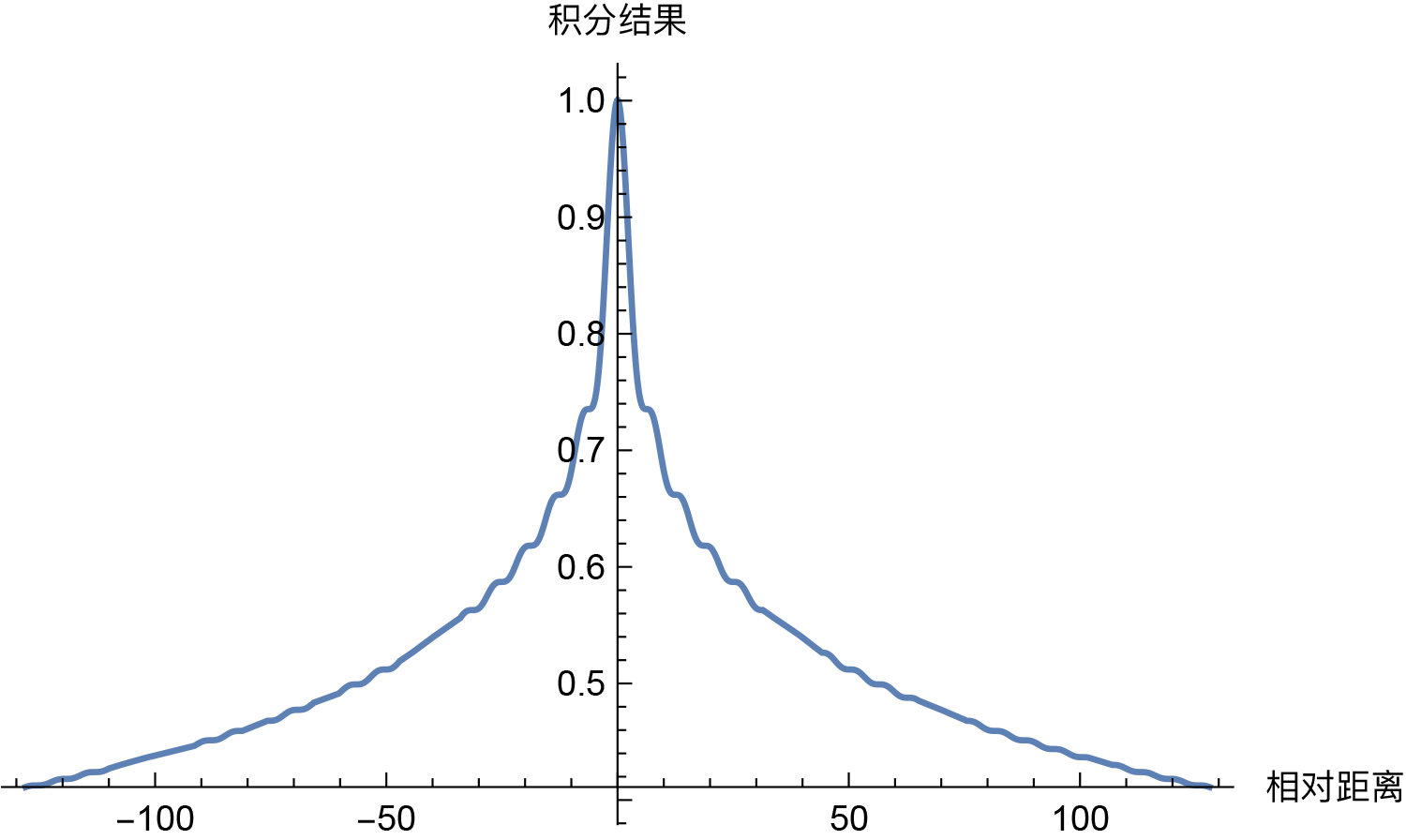
Sinusoidal 位置编码具有远程衰减的性质,具体表现为:对于两个相同的词向量,如果它们之间的距离越近,则他们的内积分数越高,反之则越低。远程衰减带来的影响是使得位置编码更倾向于捕捉局部信息,限制了远程交互的影响。这种特性对短序列有效,但对长序列可能受限,即造成 Sinusoidal 位置编码外推性一般。
二 旋转位置编码 RoPE
2.1 RoPE 算法原理
对于 RoPE 而言,作者的出发点为:通过绝对位置编码的方式实现相对位置编码。
RoPE 论文提出为了能利用 token 之间的相对位置信息($m-n$),希望 $q_m$ 和 $k$ 之间的内积,即 $f(q, m) \cdot f(k, n)$ 中能够带有相对位置信息 $m-n$。那么问题来了, $f(q, m) \cdot f(k, n)$ 的计算如何才算带有相对位置信息,论文提出只需将其能够表示成一个关于 $q$、$k$ 以及它们之间的相对位置 $m - n$ 的函数 $g(q, k, m - n)$ 即可,公式表达如下所示:
\[\langle f_q(q, m), f_k(k, n) \rangle = g(q, k, m - n) \quad (5)\]注意,这里只有 $f_q(q, m)$, $f_k(k, n)$ 是需要求解的函数,$\langle \rangle$ 表示内积操作,而对于 $g$,我们要求是表达式中有 $q, k, (m-n)$,也可以说是 $q_m, k$ 的内积会受相对位置 $m-n$ 影响。
接下来的目标就是找到一个等价的位置编码方式 $f$,从而使得上述关系成立,函数 $f_q$ 包含了位置编码和 $W_q \times q$(嵌入向量转换为 $q$ 向量)过程。
2.2 二维位置编码
假设现在词嵌入向量的维度是两维 $d=2$,这样就可以利用上 $2$ 维度平面上的向量的几何性质,论文作者借助复数来进行求解, 提出了一个满足上述关系的 $f$ 和 $g$ 的形式如下:
\[f_q(x_m, m) = (W_q x_m) e^{im\theta} \\ f_k(x_n, n) = (W_k x_n) e^{in\theta} \\ g(x_m, x_n, m - n) = Re \left[ (W_q x_m)(W_k x_n)^* e^{i(m-n)\theta} \right] \quad (6)\]其中 ( Re ) 表示复数的实部,( (W_k k)^* ) 表示 ( (W_k k) ) 的共轭复数, $x_m$ 表示第 $m$ 个 token 向量。
$f_q、f_k$ 的推导需要基于三角函数定理、欧拉公式等,推导过程参考这里,本文直接给出结论:
1,$f_q(q, m)$ 其实等于 query 向量乘以了一个旋转矩阵,即:
2,$f_k(k, n)$ 其实等于 key 向量乘以了一个旋转矩阵,即:
3,同样可得 $g(q, k, m - n)$ 等于 $q_m^T$ 乘以旋转矩阵再乘以 $k$,即:
\[\langle f_q(q, m), f_k(k, n) \rangle = \mathbf{q}_m^T R(m - n) \mathbf{k}_n \quad (9)\] \[\begin{aligned} g(q, k, m - n) &= (q_m^{(1)} k^{(1)} + q_m^{(2)} k^{(2)}) \cos((m - n)\theta) - (q_m^{(2)} k^{(1)} - q_m^{(1)} k^{(2)}) \sin((m - n)\theta) \\ &= \begin{pmatrix} q_m^{(1)} & q_m^{(2)} \end{pmatrix} \begin{pmatrix} \cos((m - n)\theta) & -\sin((m - n)\theta) \\ \sin((m - n)\theta) & \cos((m - n)\theta) \end{pmatrix} \begin{pmatrix} k_n^{(1)} \\ k_n^{(2)} \end{pmatrix} \\ &= \mathbf{q}_m^T R(m - n) \mathbf{k}_n \end{aligned} \quad(10)\]公式(9)的证明也可通过旋转矩阵性质得到,先将公式 (9) 抽象成 $\langle R_a X, R_b Y \rangle = \langle X, R_{b-a} Y \rangle$($R$ 表示旋转矩阵,$X、Y$ 表示向量), 该等式的证明过程如下:
\[\begin{aligned} \langle R_a X, R_b Y \rangle &= (R_aX)^T R_bY \\ &= X^T R_a^T R_bY \\ &= X^T R(-a)R_bY \\ &= X^T R_{(b-a)}Y = \langle X, R_{(b-a)}Y \rangle\\ \end{aligned} \quad(11)\]上述推导过程分别应用了:展开内积、矩阵乘法的结合律、旋转矩阵性质1、旋转矩阵性质2。
总结:和正弦位置编码不同,RoPE 并不是直接将位置信息 $p_i$ 和嵌入向量元素 $x_i$ 相加,而是通过与正弦函数相乘的方式引入相对位置信息。
2.3 多维的 RoPE 算法
前面的公式推导,是假设的词嵌入维度是 2 维向量,将二维推广到任意维度,$f_{{q,k}}$ 可以表示如下:
\[f_{\{q,k\}}(q, m) = R_{\Theta, m}^d W_{\{q,k\}} q \tag{12}\]其中,$R_{\Theta, m}^d$ 为 $d$ 维度的旋转矩阵,表示为:
\[R_{\Theta, m}^d = \begin{pmatrix} \cos m\theta_0 & -\sin m\theta_0 & 0 & 0 & \cdots & 0 & 0 \\ \sin m\theta_0 & \cos m\theta_0 & 0 & 0 & \cdots & 0 & 0 \\ 0 & 0 & \cos m\theta_1 & -\sin m\theta_1 & \cdots & 0 & 0 \\ 0 & 0 & \sin m\theta_1 & \cos m\theta_1 & \cdots & 0 & 0 \\ \vdots & \vdots & \vdots & \vdots & \ddots & \vdots & \vdots \\ 0 & 0 & 0 & 0 & \cdots & \cos m\theta_{d/2-1} & -\sin m\theta_{d/2-1} \\ 0 & 0 & 0 & 0 & \cdots & \sin m\theta_{d/2-1} & \cos m\theta_{d/2-1} \end{pmatrix} \tag{13}\]$R_{\Theta, m}^d$ 的形状是 [sqe_len, dim//2]。可以看出,对于 $d >= 2$ 的通用情况,则是将词嵌入向量元素按照两两一组分组,每组应用同样的旋转操作且每组的旋转角度计算方式如下:
将 RoPE 应用到前面公式(2)的 Self-Attention 计算,可以得到包含相对位置信息的Self-Attetion:
\[q_m^T k = \left( R_{\Theta, m}^d W_q q \right)^T \left( R_{\Theta, n}^d W_k k \right) = q^T W_q R_{\Theta, n-m}^d W_k k \tag{14}\]其中, \(R_{\Theta, n-m}^d = \left( R_{\Theta, m}^d \right)^T R_{\Theta, n}^d\)
Rotary Position Embedding(RoPE) 实现的可视化如下图所示:
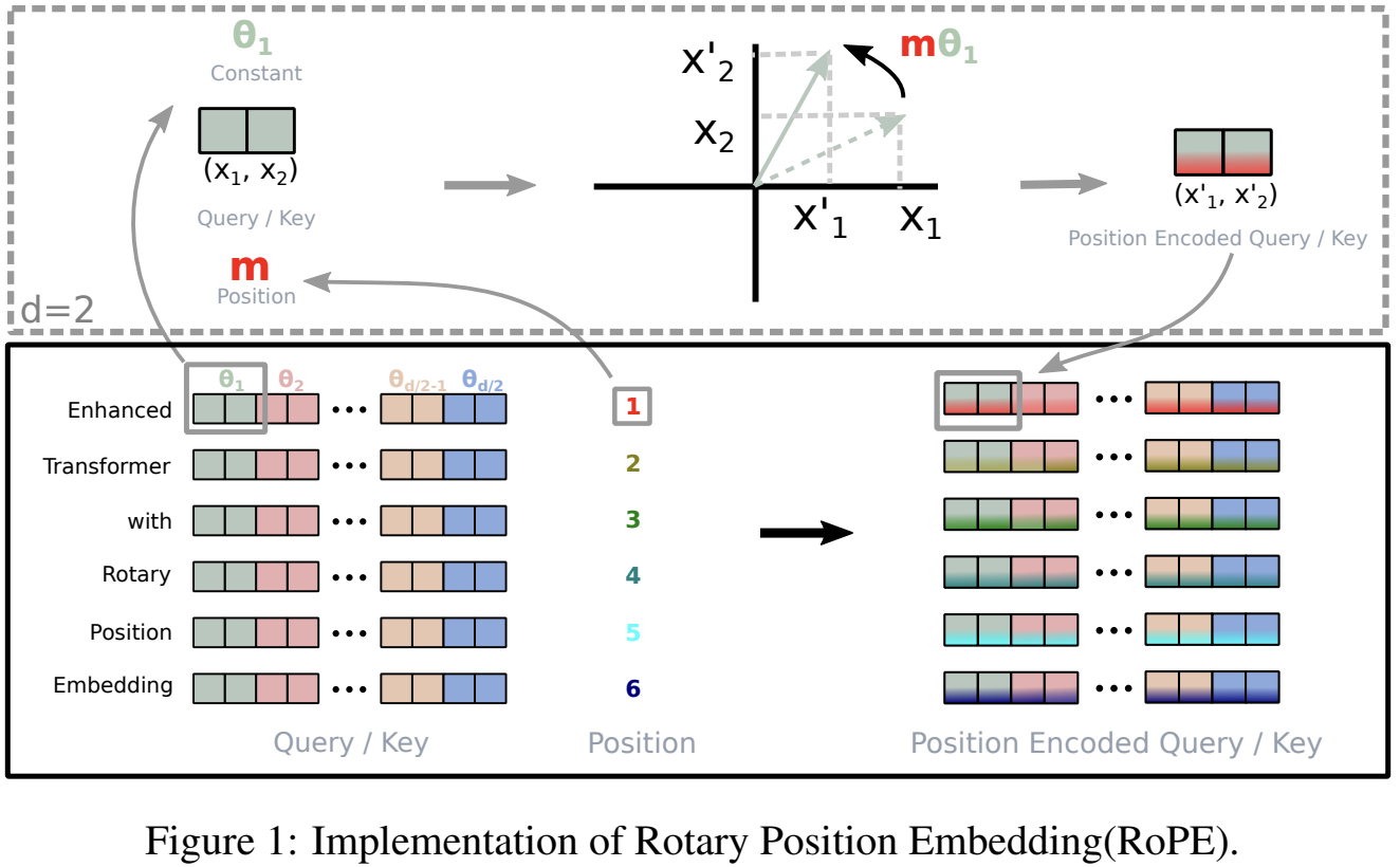
最后总结结合 RoPE 的 self-attention 操作的流程如下:
- 首先,对于
token序列中的每个词嵌入向量,都计算其对应的 query 和 key 向量; - 然后在得到 query 和 key 向量的基础上,应用前面 $f_q(q, m)$ 和 $f_k(k, n)$ 的计算公式(7)和(8)对每个
token位置都计算对应的旋转位置编码; - 接着对每个
token位置的 query 和 key 向量的元素按照两两一组应用旋转变换; - 最后再计算
query和key之间的内积得到 self-attention 的计算结果。
三 RoPE 的 pytorch 实现
3.1 RoPE 实现流程
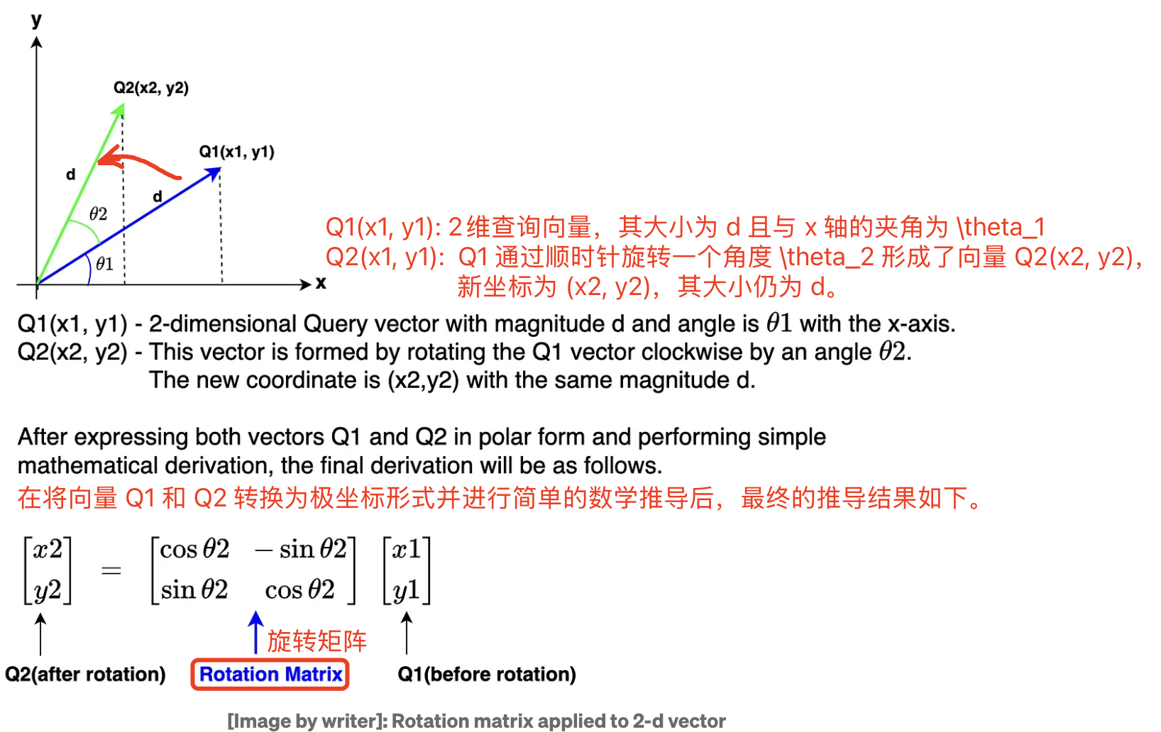
先看旋转矩阵用于旋转一个二维向量过程示例:
但是 Llama 模型的嵌入维度高达 $4096$,比二维复杂得多,如何在更高维度的嵌入上应用旋转操作呢?通过 RoPE 算法原理我们知道,嵌入向量的旋转实际是将每个嵌入向量元素位置 $m$ 的值与每一对嵌入维度对应的 $\theta$ 相乘,过程如下图所示:
RoPE 通过实现旋转矩阵,是既捕获绝对位置信息,又结合相对位置信息的方式(论文公式有更详细体现)。
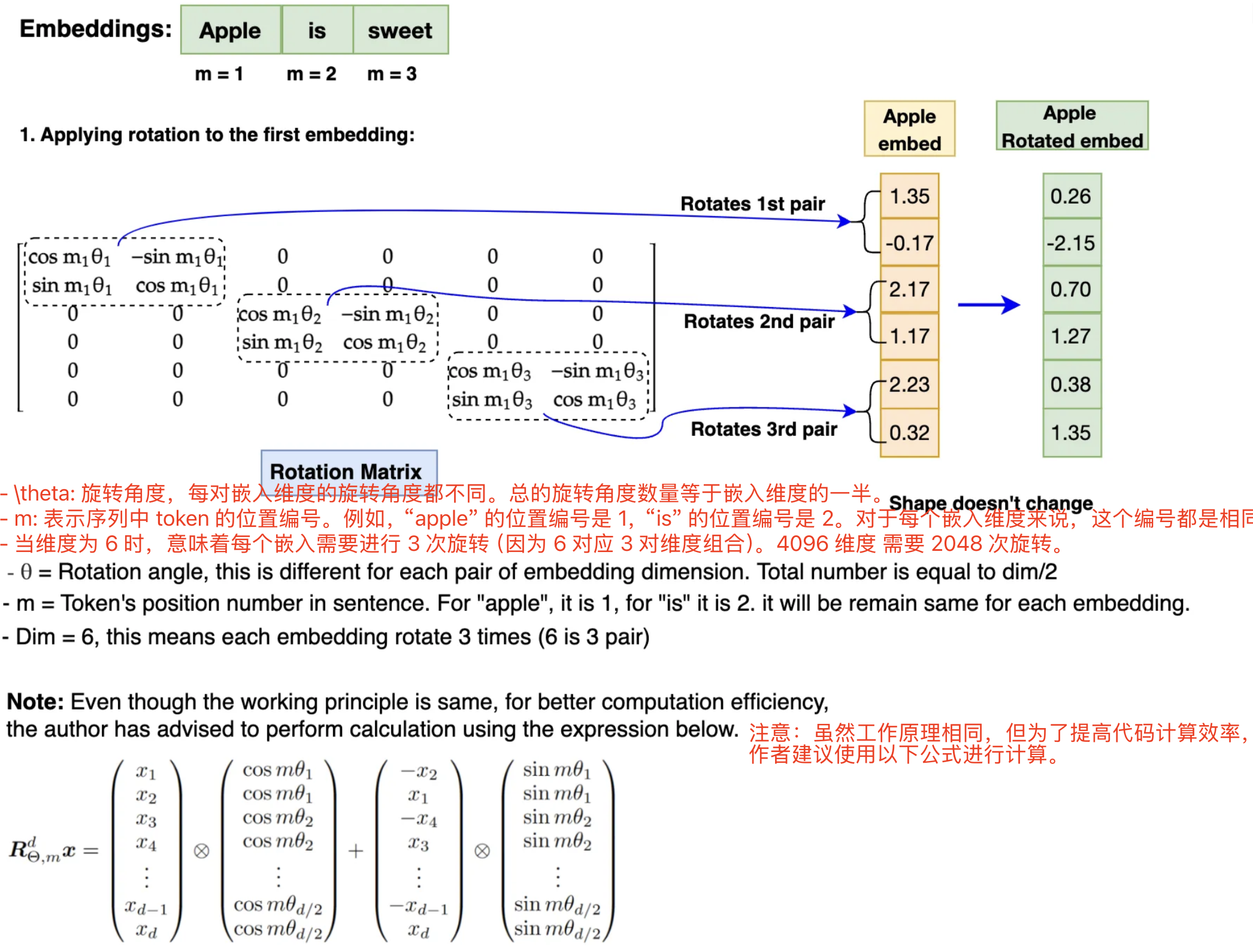
图中每组的旋转角度计算方式如下:
\[\Theta = \left\{ \theta_i = 10000^{-2(i-1)/d}, i \in [1, 2, \dots, d/2] \right\}\]在实现 RoPE 算法之前,需要注意:为了方便代码实现,在进行旋转之前,需要将旋转矩阵转换为极坐标形式,嵌入向量($q$、$k$)需要转换为复数形式。完成旋转后,旋转后的嵌入需要转换回实数形式,以便进行注意力计算。此外,RoPE 仅应用于查询(Query)和键(Key)的嵌入,不适用于值(Value)的嵌入。
3.2 RoPE 的旋转矩阵实现
Qwen3RotaryEmbedding 类如下所示,forward 用于生成旋转矩阵 cos 和 sin。
class Qwen3RotaryEmbedding(nn.Module):
    """
    用于 Qwen-3 系列模型的旋转位置编码(RoPE)张量构造器。
    该模块只负责计算 cos/sin 两张查表张量,供后续 q,k 张量做旋转。
    """
    def __init__(self, config: Qwen3Config, device: Optional[str] = None):
        super().__init__()

        # ---- ① 解析 RoPE 子类型 ----
        if hasattr(config, "rope_scaling") and config.rope_scaling is not None:
            self.rope_type = config.rope_scaling.get(
                "rope_type",  # 新字段
                config.rope_scaling.get("type", "default")  # 旧字段兜底
            )
        else:
            self.rope_type = "default"  # 若没配,则走默认实现

        # ---- ② 记录最大序列长度(缓存大小)----
        self.max_seq_len_cached = config.max_position_embeddings
        self.original_max_seq_len = config.max_position_embeddings

        # ---- ③ 保存 config 并选择初始化函数 ----
        self.config = config
        self.rope_init_fn = ROPE_INIT_FUNCTIONS[self.rope_type]

        # ---- ④ 生成 inv_freq 与缩放因子 ----
        #   inv_freq shape: (head_dim//2,),内容为 1/θ^i
        #   attention_scaling: 针对部分 RoPE 变体的额外缩放
        inv_freq, self.attention_scaling = self.rope_init_fn(config, device)

        # 注册为 buffer → 保存到 state_dict,但不算模型参数
        self.register_buffer("inv_freq", inv_freq, persistent=False)
        self.original_inv_freq = self.inv_freq  # 再存一份备份,便于动态扩展
        head_dim = config.hidden_size // config.num_attention_heads
        # 打印初始化信息
        print(f"🔧 初始化 RoPE 编码器: 类型={self.rope_type}, 最大位置={self.max_seq_len_cached}")
        print(f"  头维度={head_dim}, 频率参数形状={inv_freq.shape}, 缩放因子={self.attention_scaling}")

    # --- 前向计算 ---
    @torch.no_grad()          # 不需要梯度
    @dynamic_rope_update      # 高阶装饰器:支持在线扩展 RoPE 长度
    def forward(self, x: torch.Tensor, position_ids: torch.Tensor):
        """
        参数
        ----
        x:            (bs, seq, hidden_size) 只是用来拿 dtype/device
        position_ids: (bs, seq)              每个 token 的绝对位置

        返回
        ----
        cos, sin: 二张查表张量,shape=(bs, seq, head_dim)
        """
        # 0. 设备处理(确保在正确设备上)
        device = x.device

        # 1. 将 inv_freq 尺寸 [head_dim//2] 扩展到 (bs, head_dim//2, 1)
        inv_freq_expanded = (self.inv_freq[None, :, None]  # [1, head_dim//2, 1]
                            .float()                      # 确保fp32精度
                            .expand(position_ids.shape[0], -1, 1)  # [bs, head_dim//2, 1]
                            .to(device)) # 确保张量位于正确的计算设备上(CPU或GPU)
        print("【频率因子】inv_freq shape:", inv_freq_expanded.shape)
        print("【拓展后的频率因子】inv_freq_expanded shape:", inv_freq_expanded.shape)

        # 2. 将 position_ids (bs, seq) 扩展到 (bs, 1, seq)
        position_ids_expanded = position_ids[:, None, :].float()  # [bs, 1, seq]

        # 3. 指定 autocast 的设备类型(MPS 例外需退回 cpu)
        device_type = "cpu" if device.type == "mps" else device.type

        # 4. 强制禁用 autocast → 用 fp32 计算角度,防止精度损失
        with torch.autocast(device_type=device_type, enabled=False):
            # 矩阵乘法: [bs, head_dim//2, 1] @ (bs, 1, seq) → (bs, head_dim//2, seq)
            # 结果 freqs 张量包含了用于后续sin/cos计算的角度值。
            freqs = torch.matmul(inv_freq_expanded, position_ids_expanded)

            # 转置: (bs, head_dim//2, seq) → (bs, seq, head_dim//2)
            freqs = freqs.transpose(1, 2)

            # 拼接偶、奇维度 → (bs, seq, head_dim)
            emb = torch.cat((freqs, freqs), dim=-1)

            # 取 cos / sin(再乘可选 scaling)
            cos = emb.cos() * self.attention_scaling
            sin = emb.sin() * self.attention_scaling

        # 5. 与输入张量保持一致的 dtype 返回
        return cos.to(dtype=x.dtype), sin.to(dtype=x.dtype)
forward 函数的计算流程可视化如下所示:
graph TD
    A[inv_freq] -->|扩展维度| B[inv_freq_expanded<br>2×2×1]
    C[position_ids] -->|扩展维度| D[position_ids_expanded<br>2×1×3]
    B -->|矩阵乘法| E[freqs<br>2×2×3]
    D -->|矩阵乘法| E
    E -->|转置| F[freqs_transposed<br>2×3×2]
    F -->|复制拼接| G[emb<br>2×3×4]
    G -->|cos运算| H[cos<br>2×3×4]
    G -->|sin运算| I[sin<br>2×3×4]
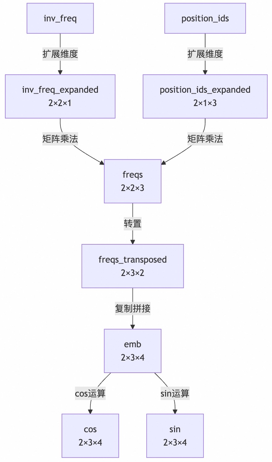
concat 拼接操作的意义体现了 RoPE 的核心设计思想:每个频率分量会同时用于生成 cos 和 sin 值,用于对应的偶数和奇数维度位置。
上述 Qwen3RotaryEmbedding 类的测试代码如下所示:
import torch
import torch.nn as nn
from typing import Optional, Tuple
import numpy as np

# 定义装饰器(如果没有动态更新需求,可以使用空装饰器)
def dynamic_rope_update(func):
    return func

# 定义RoPE初始化函数字典
ROPE_INIT_FUNCTIONS = {
    "default": lambda config, device: default_rope_init(config, device),
    # 添加其他初始化类型...
}

def default_rope_init(config, device) -> Tuple[torch.Tensor, float]:
    """默认RoPE初始化函数"""
    # 计算每个头的维度
    head_dim = config.hidden_size // config.num_attention_heads

    # 计算基础频率
    base = getattr(config, "rope_theta", 10000.0)
    inv_freq = 1.0 / (base ** (torch.arange(0, head_dim, 2, device=device).float() / head_dim))

    # 默认缩放因子为1.0
    attention_scaling = 1.0
    return inv_freq, attention_scaling

# 简化的配置类
class Qwen3Config:
    def __init__(self, rope_scaling=None, max_position_embeddings=4096,
                 hidden_size=4096, num_attention_heads=32, rope_theta=10000.0):
        self.rope_scaling = rope_scaling
        self.max_position_embeddings = max_position_embeddings
        self.hidden_size = hidden_size
        self.num_attention_heads = num_attention_heads
        self.rope_theta = rope_theta

# ===== 增强版测试函数 =====
def test_rotary_embedding(visualize: bool = True):
    """全面测试 RoPE 实现并输出详细分析"""
    print("\n" + "="*60)
    print("🔥 Qwen-3 RoPE 旋转位置编码 全面测试")
    print("="*60)

    # 配置参数
    bs, seq, n_heads, head_dim = 2, 16, 32, 128
    hidden_size = n_heads * head_dim

    print(f"\n📋 测试配置:")
    print(f"  批大小 (bs) = {bs}")
    print(f"  序列长度 (seq) = {seq}")
    print(f"  注意力头数 (n_heads) = {n_heads}")
    print(f"  每个头的维度 (head_dim) = {head_dim}")
    print(f"  总隐藏大小 (hidden_size) = {hidden_size}")

    # 创建配置对象
    dummy_cfg = Qwen3Config(
        rope_scaling={"rope_type": "default"},
        max_position_embeddings=4096,
        hidden_size=hidden_size,
        num_attention_heads=n_heads,
        rope_theta=10000.0
    )

    # 创建RoPE模块
    print("\n🛠 创建 RoPE 编码器...")
    rot = Qwen3RotaryEmbedding(dummy_cfg, device="cpu")

    # 打印频率参数信息
    inv_freq = rot.inv_freq.cpu().numpy()
    print(f"\n📊 频率参数分析 (inv_freq):")
    print(f"  形状: {inv_freq.shape}")
    print(f"  最小值: {inv_freq.min():.6f}")
    print(f"  最大值: {inv_freq.max():.6f}")
    print(f"  平均值: {inv_freq.mean():.6f}")
    print(f"  前5个值: {inv_freq[:5].round(6)}")

    # 创建测试数据
    x = torch.randn(bs, seq, hidden_size)  # 模拟输入
    position_ids = torch.arange(seq).repeat(bs, 1)  # (bs, seq)

    print("\n⚡ 计算 RoPE 编码...")
    cos, sin = rot(x, position_ids)

    # 验证输出
    print("\n✅ 输出验证:")
    print(f"  cos 形状: {cos.shape} → (批大小, 序列长度, head_dim)")
    print(f"  sin 形状: {sin.shape}")

    # 验证三角函数性质
    cos_sin_sum = cos**2 + sin**2
    error = (cos_sin_sum - 1).abs().max()
    print(f"\n🔍 数学性质验证 (cos²θ + sin²θ = 1):")
    print(f"  最大误差: {error.item():.3e}")
    print(f"  是否接近1 (误差 < 1e-6): {'是' if error < 1e-6 else '否'}")

    # 分析位置差异
    print("\n🌐 位置编码差异分析:")
    for pos_diff in [0, 1, 4, 8]:
        # 计算位置差为pos_diff时的点积
        dot_products = []
        for i in range(0, seq - pos_diff):
            q = cos[0, i] * sin[0, i + pos_diff] - sin[0, i] * cos[0, i + pos_diff]
            dot_products.append(q.mean().item())

        avg_dot = np.mean(dot_products)
        print(f"  位置差 {pos_diff:2d}: 平均点积 = {avg_dot:.4f}")

    # 可视化部分
    if visualize:
        try:
            import matplotlib.pyplot as plt
            # 1. 频率参数可视化
            plt.figure(figsize=(12, 10))

            # 频率参数
            plt.subplot(2, 1, 1)
            plt.plot(inv_freq, 'o-', markersize=3)
            plt.title("RoPE Frequency Parameters (inv_freq)")
            plt.xlabel("Dimension Index")
            plt.ylabel("Frequency Value")
            plt.grid(True)

            # 2. 不同位置的角度变化
            plt.subplot(2, 1, 2)
            positions_to_plot = [0, 1, 4, 8]
            dims_to_plot = min(32, head_dim)

            # 取第一个batch的不同位置
            for pos in positions_to_plot:
                # 计算角度 (θ = position * inv_freq)
                angles = (position_ids[0, pos] * rot.inv_freq).cpu().numpy()
                plt.plot(angles[:dims_to_plot], label=f"Position {pos}")

            plt.title(f"Angle Values for First {dims_to_plot} Dimensions")
            plt.xlabel("Dimension Index")
            plt.ylabel("Angle (radians)")
            plt.legend()
            plt.grid(True)
            plt.tight_layout()
            plt.savefig("rope_analysis.png")
            print("\n📈 可视化已保存至 rope_analysis.png")

            # 3. 位置差异热力图
            plt.figure(figsize=(10, 8))
            max_pos = 10  # 只显示前10个位置

            # 计算相对位置编码的差异
            position_diff = np.zeros((max_pos, max_pos))
            for i in range(max_pos):
                for j in range(max_pos):
                    # 计算点积作为相似度
                    sim = (cos[0, i] * cos[0, j] + sin[0, i] * sin[0, j]).mean().item()
                    position_diff[i, j] = sim

            plt.imshow(position_diff, cmap='viridis', origin='lower')
            plt.colorbar(label='Position Similarity')
            plt.title("Position Encoding Similarity Heatmap")
            plt.xlabel("Position j")
            plt.ylabel("Position i")
            plt.xticks(range(max_pos))
            plt.yticks(range(max_pos))
            plt.savefig("position_similarity.png")
            print("📊 位置相似度热力图已保存至 position_similarity.png")

        except ImportError:
            print("\n⚠ 无法导入 matplotlib,跳过可视化部分")

    print("\n🎉 测试完成!")

# 执行测试
if __name__ == "__main__":
    test_rotary_embedding(visualize=True)
上述程序运行后输出结果如下所示:
============================================================
🔥 Qwen-3 RoPE 旋转位置编码 全面测试
============================================================

📋 测试配置:
  批大小 (bs) = 2
  序列长度 (seq) = 16
  注意力头数 (n_heads) = 32
  每个头的维度 (head_dim) = 128
  总隐藏大小 (hidden_size) = 4096

🛠 创建 RoPE 编码器...
🔧 初始化 RoPE 编码器: 类型=default, 最大位置=4096
  头维度=128, 频率参数形状=torch.Size([64]), 缩放因子=1.0

📊 频率参数分析 (inv_freq):
  形状: (64,)
  最小值: 0.000115
  最大值: 1.000000
  平均值: 0.116562
  前5个值: [1.       0.865964 0.749894 0.649382 0.562341]

⚡ 计算 RoPE 编码...
inv_freq_expanded shape: torch.Size([2, 64, 1])

✅ 输出验证:
  cos 形状: torch.Size([2, 16, 128]) → (批大小, 序列长度, head_dim)
  sin 形状: torch.Size([2, 16, 128])

🔍 数学性质验证 (cos²θ + sin²θ = 1):
  最大误差: 1.192e-07
  是否接近1 (误差 < 1e-6): 是

🌐 位置编码差异分析:
  位置差  0: 平均点积 = 0.0000
  位置差  1: 平均点积 = 0.1094
  位置差  4: 平均点积 = 0.1844
  位置差  8: 平均点积 = 0.1783

📈 可视化已保存至 rope_analysis.png
📊 位置相似度热力图已保存至 position_similarity.png
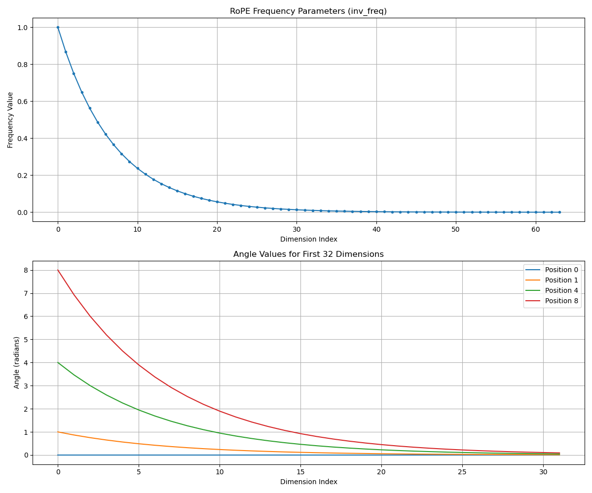
RoPE Frequency Parameters 解释:
- X轴: Dimension Index (维度索引)
- Y轴: Frequency Value (频率值)
展示频率参数随维度索引的变化
- Angle Values for First N Dimensions:
- X轴: Dimension Index (维度索引)
- Y轴: Angle (radians) (角度值,弧度)
- 不同颜色代表不同位置(0,1,4,8)在各维度的角度值
3.3 apply_rotary_pos_emb 实现
函数 f 实现拆解
得到旋转矩阵后,再应用旋转矩阵位置编码,得到集成了相对位置信息的 $q$ 和 $k$,核心公式拆解分析如下。
RoPE 的核心思想是通过旋转操作将位置信息编码到查询和键向量中。对于位置 $m$ 的查询向量 $q_m$ 和位置 $n$ 的键向量 $k_n$,旋转后的向量为:
\[\tilde{q}_m = R_m q_m \\ \tilde{k}_n = R_n k_n\]其中 $R_m$ 和 $R_n$ 是位置相关的旋转矩阵。旋转后,点积结果仅依赖于相对位置 (m-n):
\[\tilde{q}_m^T \tilde{k}_n = (R_m q_m)^T (R_n k_n) = q_m^T R_m^T R_n k_n = q_m^T R_{m-n} k_n\]代码实现逐步分析:
def rotate_half(x):
    """Rotates half the hidden dims of the input."""
    # 将最后一个维度一分为二
    x1 = x[..., : x.shape[-1] // 2]
    x2 = x[..., x.shape[-1] // 2 :]
    # 拼接 -x2 与 x1
    return torch.cat((-x2, x1), dim=-1)
上述函数实现了二维旋转矩阵的核心操作。在二维空间中,旋转矩阵为:
\[R(\theta) = \begin{bmatrix} \cos \theta & -\sin \theta \\ \sin \theta & \cos \theta \end{bmatrix}\]当应用于向量 $[x, y]$ 时:
\[R(\theta) \begin{bmatrix} x \\ y \end{bmatrix} = \begin{bmatrix} x \cos \theta - y \sin \theta \\ x \sin \theta + y \cos \theta \end{bmatrix}\]rotate_half 函数计算了旋转操作的一部分:$-y$ 和 $x$,对应旋转矩阵的第二列。
apply_rotary_pos_emb 的 pytorch 代码如下所示:
def apply_rotary_pos_emb(q, k, cos, sin, position_ids=None, unsqueeze_dim=1):
    # 调整 cos/sin 形状以匹配 q/k 的维度
    cos = cos.unsqueeze(unsqueeze_dim)  # 添加新维度
    sin = sin.unsqueeze(unsqueeze_dim)  # 添加新维度

    # 应用旋转位置嵌入到查询向量
    q_embed = (q * cos) + (rotate_half(q) * sin)

    # 应用旋转位置嵌入到键向量
    k_embed = (k * cos) + (rotate_half(k) * sin)

    return q_embed, k_embed
函数实现了完整的旋转操作:
\[\tilde{q}_m = q_m \odot \cos(m\theta) + \text{rotate\_half}(q_m) \odot \sin(m\theta)\]其中:
q * cos对应旋转矩阵的第一列操作:$x \cdot cos \theta$rotate_half(q) * sin对应旋转矩阵的第二列操作:$(-y sin \theta, x sin \theta)$
当两者相加时,就完成了完整的旋转操作:
\[\begin{bmatrix} x \cos \theta - y \sin \theta \\ x \sin \theta + y \cos \theta \end{bmatrix} = \begin{bmatrix} x \\ y \end{bmatrix} \cos \theta + \begin{bmatrix} -y \\ x \end{bmatrix} \sin \theta\]RoPE 将高维空间分解为多个二维子空间,在每个子空间上独立应用旋转:
\[R_{\Theta,m}^d = \begin{pmatrix} \cos m\theta_1 & -\sin m\theta_1 & 0 & \cdots & 0 \\ \sin m\theta_1 & \cos m\theta_1 & 0 & \cdots & 0 \\ 0 & 0 & \cos m\theta_2 & -\sin m\theta_2 & \cdots \\ \vdots & \vdots & \vdots & \ddots & \vdots \\ 0 & 0 & \cdots & \cos m\theta_{d/2} & -\sin m\theta_{d/2} \\ 0 & 0 & \cdots & \sin m\theta_{d/2} & \cos m\theta_{d/2} \end{pmatrix}\]总结
代码中通过以下方式实现这种分组处理:
- rotate_half 函数将输入向量分为前后两半
- 对每个二维子空间应用相同的旋转公式
- 不同子空间使用不同的旋转频率 $\theta_i$
测试代码
apply_rotary_pos_emb 测试代码如下所示:
import torch, math
import numpy as np

def rotate_half(x):
    """旋转输入的一半隐藏维度"""
    x1 = x[..., : x.shape[-1] // 2]
    x2 = x[..., x.shape[-1] // 2 :]
    return torch.cat((-x2, x1), dim=-1)

def apply_rotary_pos_emb(q, k, cos, sin, position_ids=None, unsqueeze_dim=1):
    cos = cos.unsqueeze(unsqueeze_dim)
    sin = sin.unsqueeze(unsqueeze_dim)
    q_embed = (q * cos) + (rotate_half(q) * sin)
    k_embed = (k * cos) + (rotate_half(k) * sin)
    return q_embed, k_embed

def test_apply_rotary_pos_emb():
    """全面测试 RoPE 应用函数并输出详细分析"""
    print("\n" + "="*90)
    print("🔥 旋转位置编码(RoPE)应用函数 - 全面测试")
    print("="*90)

    # 测试配置
    batch_size, seq_len, num_heads, head_dim = 2, 16, 32, 128
    total_params = batch_size * num_heads * seq_len * head_dim * 2

    print("\n📋 测试配置:")
    print(f"  批大小: {batch_size}")
    print(f"  序列长度: {seq_len}")
    print(f"  注意力头数量: {num_heads}")
    print(f"  头维度: {head_dim}")
    print(f"  处理参数总量: {total_params:,} (≈{total_params/1e6:.1f}M)")
    print(f"  使用 RoPE 实现: {apply_rotary_pos_emb.__name__}")

    # 创建模拟数据
    torch.manual_seed(42)

    print("\n🔧 创建测试数据...")
    q = torch.randn(batch_size, num_heads, seq_len, head_dim)
    k = torch.randn(batch_size, num_heads, seq_len, head_dim)

    print("\n📐 旋转前张量形状验证:")
    print(f"  q 形状: {q.shape} [批大小, 头数, 序列长度, 头维度]")
    print(f"  k 形状: {k.shape} [批大小, 头数, 序列长度, 头维度]")

    # 修复原始查询向量显示问题 - 确保使用正确的索引
    print("\n🔍 原始查询向量 (批次=0, 头=0, 位置=0):")
    print(f"  形状: {q[0, 0, 0].shape}")
    print(f"  前10个元素: {q[0, 0, 0][:10].numpy().round(4)}")
    print(f"  范数: {torch.norm(q[0, 0, 0]).item():.4f}")

    # 显示不同位置的向量以增强可观察性
    print("\n🔍 原始查询向量 (批次=0, 头=0, 位置=15):")
    print(f"  前10个元素: {q[0, 0, 15][:10].numpy().round(4)}")
    print(f"  范数: {torch.norm(q[0, 0, 15]).item():.4f}")

    # 创建位置编码
    print("\n⚙️ 生成位置编码...")
    cos = torch.zeros(batch_size, seq_len, head_dim)
    sin = torch.zeros(batch_size, seq_len, head_dim)

    print("\n  位置编码(旋转矩阵)形状验证:")
    print(f"  cos 形状: {cos.shape} [批大小, 序列长度, 头维度]")
    print(f"  sin 形状: {sin.shape} [批大小, 序列长度, 头维度]")

    for b in range(batch_size):
        for pos in range(seq_len):
            angle = pos * 0.1
            for d in range(head_dim):
                freq = 0.5 ** (d // 2)
                cos[b, pos, d] = math.cos(angle * freq)
                sin[b, pos, d] = math.sin(angle * freq)

    print("\n📊 位置编码示例:")
    print("  批次=0, 位置=0:")
    print(f"    cos[:10]: {cos[0, 0, :10].numpy().round(4)}")
    print(f"    sin[:10]: {sin[0, 0, :10].numpy().round(4)}")

    print("  批次=0, 位置=1:")
    print(f"    cos[:10]: {cos[0, 1, :10].numpy().round(4)}")
    print(f"    sin[:10]: {sin[0, 1, :10].numpy().round(4)}")

    # 应用旋转位置嵌入
    print("\n⚡ 应用旋转位置编码...")
    q_rot, k_rot = apply_rotary_pos_emb(q, k, cos, sin, unsqueeze_dim=1)
    print("  ✅ 旋转应用成功")

    # 增加 q_embed 和 k_embed 形状打印
    print("\n📐 旋转后张量形状验证:")
    print(f"  q_embed 形状: {q_rot.shape} [批大小, 头数, 序列长度, 头维度]")
    print(f"  k_embed 形状: {k_rot.shape} [批大小, 头数, 序列长度, 头维度]")

    # 验证输出形状
    print("\n✅ 输出验证:")
    print(f"  旋转后查询向量形状: {q_rot.shape} (应与输入相同)")
    print(f"  旋转后键向量形状: {k_rot.shape}")

    # 增强的旋转前后对比
    print("\n🔄 旋转前后对比 (批次=0, 头=0, 位置=0):")
    print("  原始向量:")
    print(f"    前10个元素: {q[0, 0, 0][:10].numpy().round(4)}")
    print(f"    范数: {torch.norm(q[0, 0, 0]).item():.4f}")

    print("  旋转后向量:")
    print(f"    前10个元素: {q_rot[0, 0, 0][:10].numpy().round(4)}")
    print(f"    范数: {torch.norm(q_rot[0, 0, 0]).item():.4f}")

    print("\n🔄 旋转前后对比 (批次=0, 头=0, 位置=15):")
    print("  原始向量:")
    print(f"    前10个元素: {q[0, 0, 15][:10].numpy().round(4)}")
    print(f"    范数: {torch.norm(q[0, 0, 15]).item():.4f}")

    print("  旋转后向量:")
    print(f"    前10个元素: {q_rot[0, 0, 15][:10].numpy().round(4)}")
    print(f"    范数: {torch.norm(q_rot[0, 0, 15]).item():.4f}")

    # 验证模长不变性
    print("\n🔍 范数保持验证:")
    max_diff = 0.0
    for b in range(batch_size):
        for h in range(num_heads):
            for pos in range(seq_len):
                orig_norm = torch.norm(q[b, h, pos]).item()
                rot_norm = torch.norm(q_rot[b, h, pos]).item()
                diff = abs(orig_norm - rot_norm)
                max_diff = max(max_diff, diff)

    print(f"  最大范数差异: {max_diff:.6f}")
    if max_diff < 1e-5:
        print("  ✅ 通过: 所有向量范数保持稳定 (<1e-5)")
    else:
        print(f"  ⚠ 警告: 某些位置的范数差异超出容差范围 (最大差异 = {max_diff:.6f})")

    # 验证相对位置性质
    print("\n🌐 相对位置特性验证:")
    print("  计算位置0与其他位置的相似度...")
    print("  (RoPE中,相似度应随位置差增大而减小)")

    print("\n  位置对 | 相似度 | 与前一位置差异")
    print("  -------|--------|-----------------")

    prev_sim = None
    for pos_diff in [0, 1, 2, 4, 8]:
        if seq_len > pos_diff:
            dot_product = (q_rot[0, 0, 0] @ q_rot[0, 0, pos_diff]).item()

            diff_str = ""
            if prev_sim is not None:
                diff = prev_sim - dot_product
                diff_str = f"{diff:+.6f}" if diff > 0 else f"{diff:.6f}"

            print(f"  0 vs {pos_diff:2d} | {dot_product:.6f} | {diff_str}")
            prev_sim = dot_product

# 执行测试
if __name__ == "__main__":
    test_apply_rotary_pos_emb()
程序运行后输出结果如下所示:
==========================================================================================
🔥 旋转位置编码(RoPE)应用函数 - 全面测试
==========================================================================================

📋 测试配置:
  批大小: 2
  序列长度: 16
  注意力头数量: 32
  头维度: 128
  处理参数总量: 262,144 (≈0.3M)
  使用 RoPE 实现: apply_rotary_pos_emb

🔧 创建测试数据...

📐 旋转前张量形状验证:
  q 形状: torch.Size([2, 32, 16, 128]) [批大小, 头数, 序列长度, 头维度]
  k 形状: torch.Size([2, 32, 16, 128]) [批大小, 头数, 序列长度, 头维度]

🔍 原始查询向量 (批次=0, 头=0, 位置=0):
  形状: torch.Size([128])
  前10个元素: [ 1.9269  1.4873  0.9007 -2.1055  0.6784 -1.2345 -0.0431 -1.6047 -0.7521
  1.6487]
  范数: 10.8772

🔍 原始查询向量 (批次=0, 头=0, 位置=15):
  前10个元素: [ 0.5484  0.4577  0.9677 -0.6674  1.6183 -0.2644  1.3541 -0.0709 -0.3697
 -0.246 ]
  范数: 10.4785

⚙️ 生成位置编码...

  位置编码(旋转矩阵)形状验证:
  cos 形状: torch.Size([2, 16, 128]) [批大小, 序列长度, 头维度]
  sin 形状: torch.Size([2, 16, 128]) [批大小, 序列长度, 头维度]

📊 位置编码示例:
  批次=0, 位置=0:
    cos[:10]: [1. 1. 1. 1. 1. 1. 1. 1. 1. 1.]
    sin[:10]: [0. 0. 0. 0. 0. 0. 0. 0. 0. 0.]
  批次=0, 位置=1:
    cos[:10]: [0.995  0.995  0.9988 0.9988 0.9997 0.9997 0.9999 0.9999 1.     1.    ]
    sin[:10]: [0.0998 0.0998 0.05   0.05   0.025  0.025  0.0125 0.0125 0.0062 0.0062]

⚡ 应用旋转位置编码...
  ✅ 旋转应用成功

📐 旋转后张量形状验证:
  q_embed 形状: torch.Size([2, 32, 16, 128]) [批大小, 头数, 序列长度, 头维度]
  k_embed 形状: torch.Size([2, 32, 16, 128]) [批大小, 头数, 序列长度, 头维度]

✅ 输出验证:
  旋转后查询向量形状: torch.Size([2, 32, 16, 128]) (应与输入相同)
  旋转后键向量形状: torch.Size([2, 32, 16, 128])

🔄 旋转前后对比 (批次=0, 头=0, 位置=0):
  原始向量:
    前10个元素: [ 1.9269  1.4873  0.9007 -2.1055  0.6784 -1.2345 -0.0431 -1.6047 -0.7521
  1.6487]
    范数: 10.8772
  旋转后向量:
    前10个元素: [ 1.9269  1.4873  0.9007 -2.1055  0.6784 -1.2345 -0.0431 -1.6047 -0.7521
  1.6487]
    范数: 10.8772

🔄 旋转前后对比 (批次=0, 头=0, 位置=15):
  原始向量:
    前10个元素: [ 0.5484  0.4577  0.9677 -0.6674  1.6183 -0.2644  1.3541 -0.0709 -0.3697
 -0.246 ]
    范数: 10.4785
  旋转后向量:
    前10个元素: [-0.6945  0.301   0.4007 -0.5162  1.5313 -0.3407  1.2414  0.2079 -0.247
 -0.3272]
    范数: 10.4008

🔍 范数保持验证:
  最大范数差异: 0.487347
  ⚠ 警告: 某些位置的范数差异超出容差范围 (最大差异 = 0.487347)

🌐 相对位置特性验证:
  计算位置0与其他位置的相似度...
  (RoPE中,相似度应随位置差增大而减小)

  位置对 | 相似度 | 与前一位置差异
  -------|--------|-----------------
  0 vs  0 | 118.314240 |
  0 vs  1 | 20.345375 | +97.968864
  0 vs  2 | -4.198829 | +24.544204
  0 vs  4 | 8.441195 | -12.640023
  0 vs  8 | -8.702080 | +17.143274