LLM 量化-AWQ 代码深入剖析
Categories: Model_Quant_Compression
一 llm-awq 代码架构
1.1 如何使用
作者提供了 llm-awq 仓库,开源包括了量化算法、量化模型转换和量化模型推理的代码,另外提供了 entry.py 代码来调用模型权重量化和量化推理接口。
1,获取模型权重缩放(放大)的 scale 因子,定义 args.run_awq 参数后 entry 会调用 run_awq 函数获取缩放因子 $s$,通过 --dump_awq 参数指定缩放后的 llm 权重文件路径。
python -m awq.entry --model_path /PATH/TO/LLAMA3/llama3-8b \
    --w_bit 4 --q_group_size 128 \
    --run_awq --dump_awq awq_cache/llama3-8b-w4-g128.pt
2,使用伪量化推理在 WikiText-2 数据集上评估量化模型的精度,这点对于没有实现自定义量化 kernel 的新模型想实验下 awq 量化算法在其上的效果如何还是很有用的!定义参数 args.q_backend == "fake" 后,entry 会调用 quantizer.py 的 调用 pseudo_quantize_model_weight 来执行权重伪量化操作,当然前面得先通过 apply_awq 函数应用模型权重量化因子结果 awq_results 到模型中。
python -m awq.entry --model_path /PATH/TO/LLAMA3/llama3-8b \
    --tasks wikitext \
    --w_bit 4 --q_group_size 128 \
    --load_awq awq_cache/llama3-8b-w4-g128.pt \
    --q_backend fake
3,直接将浮点模型转换为 int4 位宽的量化模型权重,转换后模型权重体积直接减小了 4 倍,定义参数 args.q_backend == "real" 后,entry 会调用 quantizer.py 的 real_quantize_model_weight() 函数将模型的浮点权重参数原地转换为量化参数,同样 entry.py代码中前面会先通过 apply_awq 函数应用模型权重量化因子结果 awq_results 到模型中。
mkdir quant_cache
python -m awq.entry --model_path /PATH/TO/LLAMA3/llama3-8b \
    --w_bit 4 --q_group_size 128 \
    --load_awq awq_cache/llama3-8b-w4-g128.pt \
    --q_backend real --dump_quant quant_cache/llama3-8b-w4-g128-awq.pt
4,真正的量化模型推理并评估精度,其中量化 kernel 的实现是作者基于 FT 框架做了些调整迁移到 awq/kernels/csrc/quantization 中,包括 gemm 和 gemv 两种 int4 矩阵乘法。
python -m awq.entry --model_path /PATH/TO/LLAMA3/llama3-8b \
    --tasks wikitext \
    --w_bit 4 --q_group_size 128 \
    --load_quant quant_cache/llama3-8b-w4-g128-awq.pt
1.2 算法代码架构
通过 entry 的四种用法可以发现,awq 仓库的算法架构和 smoothquant 很像,伪量化推理过程比较简单这里忽略,量化模型推理的实现是通过下述步骤(模块):
- 基于校准集得到激活再根据量化算法计算量化缩放因子 $s$;
- 裁剪线性层权重的最小、最大值,推测是为了抑制权重的异常值(smoothquant 没有这步);
- 在前面得到权重缩放因子 $s$ 基础上,将浮点模型权重转换为
int4量化模型权重; - 自定义 int4 矩阵乘法 kernel,并替换掉原来的浮点线性层,得到量化模型,再执行真正的量化模型推理(forward)。
在代码实现上:
- 步骤 1 的实现对应代码文件 auto_scale.py;
- 步骤 2 的实现对应 auto_clip.py;
- 步骤 3 的实现对应
pre_quant.py和 quantizer.py,前者分别调用 auto_scale.py 的apply_scale函数和 auto_clip.py 的apply_clip函数得到 awq 量化算法的最终结果awq_results给后续 quantizer.py 的模型量化函数real_quantize_model_weight用。
# awq_results 是一个字典
awq_results = {
        "scale": [],
        "clip": [],
    }
awq 的浮点模型权重量化转换是单独在
quantizer.py中实现,这点跟 smoothquant 仓库不一样,smoothquant 是将模型权重转换为量化模型推理在一个文件中通过量化类的from_float和forward(调用量化 kernel 接口) 函数来实现。
awq 代码文件组织情况如下所示,可以看出代码架构真的简单清晰,让人阅读起来很舒服!
├── entry.py           # 用户使用入口文件
├── kernels            # cuda 实现的 kernel 代码目录,包括 fp16 和 int4 的 gemm 和 gemv
│   ├── csrc
│   └── setup.py
├── quantize           # awq 算法实现目录
│   ├── __init__.py
│   ├── auto_clip.py
│   ├── auto_scale.py
│   ├── pre_quant.py
│   ├── qmodule.py
│   └── quantizer.py
└── utils              # 公共接口函数目录
    ├── __init__.py
    ├── calib_data.py
    ├── lm_eval_adaptor.py
    ├── module.py
    ├── parallel.py
    └── utils.py
不愧是同一个作者,awq 跟 smoothquant 代码仓库风格还是很统一的。
二 基于激活感知的权重放大和裁剪
2.1 auto_scale.py
auto_scale.py 是 awq 代码和 smoothquant 等量化算法代码的最大不同之一,它对应的原理和公式是论文的 3.2 节内容。
先看下 auto_scale.py 拥有的函数,其中 apply_scale() 是提供给外部模块调用的接口。

其中 scale_ln_fcs、scale_gelu_fc、scale_fc_fc 函数都是在给定缩放因子 $s$ 的前提下去缩放网络层权重参数:
scale_ln_fcs: 函数针对 ln->fcs 连接的线性层列表权重和 ln 的权重及偏置。scale_gelu_fc: 函数用于对GELU激活函数后接全连接层的权重进行缩放操作。scale_fc_fc: 函数用于缩放两个连续全连接层 fc1->fc2 权重的函数。
其中带注释的 scale_gelu_fc 函数实现如下所示:
@torch.no_grad()
def scale_gelu_fc(gelu, fc, scales):
    # 进行网络层类型检查
    assert isinstance(gelu, (nn.GELU, BloomGelu, GELUActivation))
    assert isinstance(fc, nn.Linear)

    # scales.view(1, -1) 将缩放因子重塑为 2D 张量, 以匹配权重矩阵的维度
    # mul_ 是就地乘法操作(节省内存),直接修改 fc.weight 的值
    fc.weight.mul_(scales.view(1, -1).to(fc.weight.device))

    # 遍历全连接层的所有参数,确保没有任何参数变成 NaN 值,这是一个重要的数值稳定性检查。
    for p in fc.parameters():
        assert torch.isnan(p).sum() == 0
前面论文的解读文章中,我们已经知道了权重缩放系数 $s$ 的计算公式是如下所示:
\[s = \text{mean(abs}({\mathbf{x}}))^{\alpha}, \quad \alpha^* = \arg\min_{\alpha} \mathcal{L}(\text{mean(abs}({\mathbf{x}}))^{\alpha}) \tag{5}\]其中 $\text{mean(abs}({\mathbf{x}}))$ 是逐通道计算的激活值绝对值的平均值,对应的代码实现是 auto_scale.py/get_act_scale 函数。
@torch.no_grad()
def get_act_scale(x):
    # x.abs().view(-1, x.shape[-1]): 重塑张量维度 -> [b*s, h]
    # x.abs().view(-1, x.shape[-1]).mean(0): 沿着第0维计算平均值 -> [h,]
    return x.abs().view(-1, x.shape[-1]).mean(0)
公式(5)也就是 $s$ 的自动搜索算法实现是在 _search_module_scale 函数中,代码如下所示:
# _search_module_scale 是 auto_scale_block 内的函数
def _search_module_scale(block, linears2scale: list, x, kwargs={}):
    """
    在给定的模块和输入特征下,搜索最佳的缩放因子。

    参数:
        block (nn.Module): 当前要搜索缩放因子的模块。
        linears2scale (list of nn.Linear): 需要缩放的全连接层列表。
        x (torch.Tensor): 输入特征张量。
        kwargs (dict): 其他关键字参数。

    返回:
        torch.Tensor: 最佳缩放因子,形状为 [out_features]。
    """
    x = x.to(next(block.parameters()).device)  # 将输入特征移动到模块所在设备
    with torch.no_grad():
        org_out = block(x, **kwargs)  # 原始输出
        if isinstance(org_out, tuple):
            org_out = org_out[0]

    x_max = get_act_scale(x)  # 获取激活的缩放因子

    best_error = float("inf")
    best_ratio = -1
    best_scales = None

    n_grid = 20  # 缩放比例的网格大小
    history = []  # 保存每个比例的误差

    # 保存原始状态字典
    org_sd = {k: v.cpu() for k, v in block.state_dict().items()}

    for ratio in range(n_grid):
        ratio = ratio * 1 / n_grid  # 当前比例
        scales = x_max.pow(ratio).clamp(min=1e-4).view(-1)  # s^alpha 计算缩放因子
        scales = scales / (scales.max() * scales.min()).sqrt()  # 归一化缩放因子(论文没有描述这步操作)

        for fc in linears2scale:
            # 权重乘以缩放因子,对显著权重进行放大以降低量化误差, 对应公式(2)中的 w*s
            fc.weight.mul_(scales.view(1, -1).to(fc.weight.device))
            # 使用权重量化函数 w_quantize_func 执行权重量化操作,对应公式(4) W⋅diag(s))(diag(s)^−1
            fc.weight.data = w_quantize_func(fc.weight.data) / (scales.view(1, -1))

        out = block(x, **kwargs)  # 量化后的输出
        if isinstance(out, tuple):
            out = out[0]

        # 计算均方误差
        loss = ( (org_out - out).float().pow(2).mean().item() )
        history.append(loss)

        # 如果当前误差小于最佳误差,更新最佳误差和最佳比例
        is_best = loss < best_error
        if is_best:
            best_error = loss
            best_ratio = ratio
            best_scales = scales

        # 恢复原始状态字典
        block.load_state_dict(org_sd)

    if best_ratio == -1:
        print(history)
        raise Exception("Failed to find a suitable scaling ratio.")

    best_scales = best_scales.view(-1)  # 调整形状

    assert torch.isnan(best_scales).sum() == 0, "缩放因子包含NaN值"
        return best_scales.detach()
这里我重点提下缩放因子 $s$、权重的缩放(乘以缩放因子)和权重的量化操作的实现,具体来说流程是这样的:
- 通过公式 $s = \text{mean(abs}({\mathbf{x}}))^{\alpha}$ 来得到权重的缩放因子 $s$,其中 $\alpha$ 取值范围为 0, 0.05, 0.10, 0.15 ……;
- 将权重和缩放因子相乘,实现对显著权重进行放大的目的;
- 通过指定量化函数 w_quantize_func 量化权重,注意要将激活的缩放操作融合进来,即 $Q(\mathbf{W} \cdot \text{diag}(\mathbf{s})) (\text{diag} \mathbf{s})^{-1}$。
对应代码如下所示:
scales = x_max.pow(ratio).clamp(min=1e-4).view(-1)  # 计算缩放因子
scales = scales / (scales.max() * scales.min()).sqrt()  # 为防止 scales 过大或过小,需要多一步归一化操作

# n_grid 取值 20
for ratio in range(n_grid):
    ratio = ratio * 1 / n_grid  # 当前比例
    for fc in linears2scale:
        # 权重乘以缩放因子,对显著权重进行放大以降低量化误差, 对应公式(2)中的 w*s
        fc.weight.mul_(scales.view(1, -1).to(fc.weight.device))
        # 使用权重量化函数 w_quantize_func 执行权重量化操作,对应公式(4) W⋅diag(s))(diag(s)^−1
        fc.weight.data = w_quantize_func(fc.weight.data) / (scales.view(1, -1))
另外,跟 smoothquant 不同,awq 中需要根据模块类型,分别处理不同的线性层组,即分开计算不同模块的权重缩放因子!具体来说,作者将 llm 模型分成以下几个模块分别计算 scales。
对于 OPTDecoderLayer
- self-attention 的查询、键、值投影层
- self-attention 的输出投影层
- mlp 的 第一个全连接层
- mlp 的 第二个全连接层
对于 LlamaDecoderLayer
- self-attention 的查询、键、值投影层
- self-attention 的输出投影层
- mlp 的 gate_proj 和 up_proj 线性层
- mlp 的 down_proj 线性层
其中获取 LlamaDecoderLayer 缩放因子的代码如下所示:
# 处理 LlamaDecoderLayer 的层
if isinstance(module, LlamaDecoderLayer):

    # 处理 self-attention 的查询、键、值投影层
    scales_list.append(
        # `_auto_get_scale` 是对 `_search_module_scale` 的一层包装,作用是获取某个层组的缩放因子。
        _auto_get_scale(
            prev_op=module.input_layernorm,
            layers=[
                module.self_attn.q_proj,
                module.self_attn.k_proj,
                module.self_attn.v_proj,
            ],
            inp=input_feat["self_attn.q_proj"],
            module2inspect=module.self_attn,
            kwargs=module_kwargs,
        )
    )
    # 处理 self-attention 的输出投影层
    if module.self_attn.v_proj.weight.shape == module.self_attn.o_proj.weight.shape:
        scales_list.append(
            _auto_get_scale(
                prev_op=module.self_attn.v_proj,
                layers=[module.self_attn.o_proj],
                inp=input_feat["self_attn.o_proj"],
            )
        )
    scales_list.append(
        _auto_get_scale(
            prev_op=module.post_attention_layernorm,
            layers=[module.mlp.gate_proj, module.mlp.up_proj],
            inp=input_feat["mlp.gate_proj"],
            module2inspect=module.mlp,
        )
    )
    scales_list.append(
        _auto_get_scale(
            prev_op=module.mlp.up_proj,
            layers=[module.mlp.down_proj],
            inp=input_feat["mlp.down_proj"],
        )
    )
apply_scale 函数也是对 _search_module_scale 的调用,作用是将计算得到的缩放因子应用到指定模块的层上,代码比较简单,不再分析,这里给出它的参数解释:
module: 需要应用缩放的模块。scales_list: 由 auto_scale_block 返回的缩放因子列表。input_feat_dict: 输入特征的字典,用于进一步调整输入张量。
2.2 auto_clip.py
auto_clip.py 文件提供给外界的接口是 apply_clip(module, clip_list) 函数,它的主要作用是,将裁剪最大值并应用到指定模块的全连接层权重,这块代码的原理我查了很多资料都没找到对它的分析和解释,最后又去看仔细看论文,找到了这样一句话:”We further apply weight clipping to minimize the MSE error of quantization. “ 意思是作者进一步应用了权重值裁剪方法以减少量化的均方误差 (MSE),但是为什么要这么做作者没提。
获取裁剪权重的最大值,在代码实现上本质也是一种暴力搜索 + 最小化 MSE 损失的算法,其权重最大值的获取也是通过最小 MSE 损失来求得,但这里不仅遍历了每个通道的最大值,内层循环里面还遍历了前面提到的 $\alpha$ 值,是双重循环求最小 $MSE$ 损失!
auto_clip 的实现和应用我觉得很神奇,理论层面不理解为什么要这么做,只能基于 smoothquant 论文的灵感来给出一点我的推测,个人觉得这是为了直接剔除权重中的异常值,我们都知道激活中有异常值,那么权重中也是可能存在的,自然也需要剔除,尤其是这里权重量化位宽是 INT4,如果原来的浮点值有异常值,那么很可能会影响模型精度,毕竟 INT4/INT3 或者更低位宽表示的范围跟原来的 FP16 比差别很大!
因为没找到相关理论说明,所以这里我只能先假定它是实验指导理论,后续有看到解释再来更新,直接看其代码实现吧。
# Weight Quantization: 自动裁剪层权重以适应量化
@torch.no_grad()
def auto_clip_layer(
    w, input_feat, n_bit, q_config, n_grid=20, max_shrink=0.5, n_sample_token=512
):
    """
    自动裁剪层权重以最小化量化误差。

    参数:
        w (torch.Tensor): 权重矩阵,形状为 [out_features, in_features]。
        input_feat (torch.Tensor): 输入特征,形状为 [n_token, in_features]。
        n_bit (int): 量化位数,例如8表示INT8量化。
        q_config (dict): 量化配置参数,例如 {"q_group_size": 128}。
        n_grid (int): 搜索缩放比例的网格大小,默认20。
        max_shrink (float): 最大缩放比例,默认为0.5。
        n_sample_token (int): 采样的token数量,默认512。

    返回:
        torch.Tensor: 最佳的最大裁剪值,形状为 [out_features, n_group]。
    """
    assert w.dim() == 2, "权重矩阵必须是二维的"
    org_w_shape = w.shape  # 原始权重形状

    # 获取分组大小,如果q_group_size > 0则使用该值,否则使用权重的列数
    group_size = (
        q_config["q_group_size"] if q_config["q_group_size"] > 0 else w.shape[1]
    )

    # 调整输入特征的形状
    input_feat = input_feat.view(-1, input_feat.shape[-1])  # [n_token, in_features]
    input_feat = input_feat.reshape(1, input_feat.shape[0], -1, group_size)  # [1, n_token, n_group, group_size]
    input_feat = input_feat[:, 0 :: input_feat.shape[1] // n_sample_token]  # 采样输入特征
    w = w.reshape(w.shape[0], 1, -1, group_size)  # [out_features, 1, n_group, group_size]

    # 定义每个批次处理的输出通道数,防止显存溢出
    oc_batch_size = 256 if w.shape[0] % 256 == 0 else 64
    assert w.shape[0] % oc_batch_size == 0, "输出通道数必须是 oc_batch_size 的倍数"

    w_all = w  # 保存所有权重
    best_max_val_all = []  # 保存所有批次的最佳最大值

    # 遍历每个输出通道批次
    for i_b in range(w.shape[0] // oc_batch_size):
        # 获取当前批次的权重
        w_batch = w_all[i_b * oc_batch_size : (i_b + 1) * oc_batch_size]

        # 计算每个输出通道的原始最大绝对值
        org_max_val = w_batch.abs().amax(dim=-1, keepdim=True)  # [oc_batch_size, 1, n_group, 1]

        best_max_val = org_max_val.clone()  # 初始化最佳最大值为原始最大值
        min_errs = torch.ones_like(org_max_val) * 1e9  # 初始化最小误差为很大的值
        input_feat = input_feat.to(w_batch.device)  # 将输入特征移动到权重所在设备

        # 计算原始输出
        org_out = (input_feat * w_batch).sum(dim=-1)  # [oc_batch_size, n_token, n_group]

        # 遍历缩放比例网格
        for i_s in range(int(max_shrink * n_grid)):
            # 计算当前缩放比例
            shrink_ratio = 1 - i_s / n_grid
            max_val = org_max_val * shrink_ratio  # 缩放后的最大值
            min_val = -max_val  # 对称最小值

            # 裁剪权重
            cur_w = torch.clamp(w_batch, min_val, max_val)

            # 量化权重
            q_w = pseudo_quantize_tensor(cur_w, n_bit=n_bit, **q_config)

            # 计算量化后的输出
            cur_out = (input_feat * q_w).sum(dim=-1)

            # 计算量化误差(均方误差)
            err = (cur_out - org_out).pow(2).mean(dim=1).view(min_errs.shape)  # [oc_batch_size, 1, n_group, 1]

            # 更新最小误差和最佳最大值
            cur_best_idx = err < min_errs
            min_errs[cur_best_idx] = err[cur_best_idx]
            best_max_val[cur_best_idx] = max_val[cur_best_idx]

            # 释放不再需要的张量
            del cur_w
            del cur_out

        # 保存当前批次的最佳最大值
        best_max_val_all.append(best_max_val)

    # 合并所有批次的最佳最大值
    best_max_val = torch.cat(best_max_val_all, dim=0)  # [out_features, 1, n_group, 1]

    # 清理内存
    del input_feat
    del org_out
    gc.collect()
    torch.cuda.empty_cache()

    # 返回最佳最大值,去除多余的维度
    return best_max_val.squeeze(1)  # [out_features, n_group]
需要注意的是,apply_clip(module, clip_list) 函数是应用在 apply_scale(module, scales_list) 之后的!
三 权重量化
3.1 pre_quant.py
pre_quant.py 实现了 get_named_linears、get_blocks、move_embed、run_awq 和 apply_awq 函数,其中前三个都是文件内部使用的接口,后面两个是对外提供使用的。
run_awq:运行 AWQ(自动权重量化)流程,对模型进行权重量化。apply_awq: 其实就是先后调用 apply_scale 和 apply_clip 函数,将 AWQ 权重缩放结果应用到模型中,在加载模型权重缩放因子文件后用得到。
run_awq 函数的实现逻辑相对简单,就是使用钩子函数,在跑模型推理的时候逐层获取缩放因子 scales_list 和 裁剪最大值 clip_list 结果,并调用相关 apply 函数来执行对显著权重进行放大和对权重异常值裁剪的操作。代码如下所示(做了精简):
@torch.no_grad()
def run_awq():
    # 逐层处理模型
    for i in tqdm.tqdm(range(len(layers)), desc="Running AWQ..."):
        layer = layers[i]
        layer = layer.cuda()
        named_linears = get_named_linears(layer)

        # 定义一个钩子,用于缓存所有线性层的输入特征
        def cache_input_hook(m, x, y, name, feat_dict):
            x = x[0]
            x = x.detach().cpu()
            feat_dict[name].append(x)

        input_feat = defaultdict(list)
        handles = []
        for name in named_linears:
            handles.append(
                named_linears[name].register_forward_hook(
                    functools.partial(cache_input_hook, name=name, feat_dict=input_feat)
                )
            )
        inps = inps.to(next(layer.parameters()).device)  # 确保输入在正确的设备上
        # 获取输出作为下一层的输入
        inps = layer(inps, **layer_kwargs)[0]
        for h in handles:
            h.remove()

        # 将所有输入特征拼接
        input_feat = {k: torch.cat(v, dim=0) for k, v in input_feat.items()}
        ###省略代码####
        scales_list = auto_scale_block(layer, layer_kwargs, w_bit=w_bit,q_config=q_config, input_feat=input_feat,)
        apply_scale(layers[i], scales_list, input_feat_dict=input_feat)

        clip_list = auto_clip_block(layer,w_bit=w_bit,q_config=q_config,input_feat=input_feat,)
        apply_clip(layer, clip_list)
3.2 quantizer.py
该模块文件实现了 4 个函数,后面两个是对外提供的接口,其作用如下:
- scale_activations:替换模块中的激活函数为 ScaledActivation,初始化缩放因子为1。
- pseudo_quantize_tensor:伪量化函数,将浮点数权重量化为低位整数,再反量化回浮点数。
- pseudo_quantize_model_weight: 伪量化模型中的权重,将所有线性层的权重量化。
- real_quantize_model_weight:实际量化模型中的权重,将线性层替换为量化线性层(WQLinear)。
real_quantize_model_weight 的实现流程如下所示:
- 确保只支持 zero_point 量化。
- 获取模型中的所有 Transformer 块。
- 遍历每个块,获取其中所有命名的线性层。
- 对每个线性层:
- 如果 init_only 为 True,使用 WQLinear.from_linear 初始化量化线性层,并并调用
set_op_by_name替换原有线性层。 - 否则,伪量化权重,获取缩放因子和零点,并使用 WQLinear.from_linear 初始化量化线性层(带有缩放和零点)。
- 如果 init_only 为 True,使用 WQLinear.from_linear 初始化量化线性层,并并调用
real_quantize_model_weight 函数中最关键的操作就是使用量化线性层 WQLinear 替换原来的线性层。
AWQ 的(伪)权重量化函数的和 smoothquant 略有区别,其基于 min_max + 非线性量化算法,计算量化 scale 和 zero_point,同时默认使用分组量化(即 per-group 量化,group_size 大小通过函数参数传入),核心代码如下所示:
def pseudo_quantize_tensor(
    w, n_bit=8, zero_point=True, q_group_size=-1, inplace=False, get_scale_zp=False
):
    org_w_shape = w.shape
    if q_group_size > 0:
        assert org_w_shape[-1] % q_group_size == 0
        # num_groups = weight.shape[1] // group_size
        w = w.reshape(-1, q_group_size) # 权重分组
    assert w.dim() == 2
    if zero_point:
        max_val = w.amax(dim=1, keepdim=True)
        min_val = w.amin(dim=1, keepdim=True)
        max_int = 2**n_bit - 1
        min_int = 0
        scales = (max_val - min_val).clamp(min=1e-5) / max_int
        zeros = (-torch.round(min_val / scales)).clamp_(min_int, max_int)
    else:  # we actually never used this
        assert min_val is None
        max_val = w.abs().amax(dim=1, keepdim=True)
        max_val = max_val.clamp(min=1e-5)
        max_int = 2 ** (n_bit - 1) - 1
        min_int = -(2 ** (n_bit - 1))
        scales = max_val / max_int
        zeros = 0

    assert torch.isnan(scales).sum() == 0
    assert torch.isnan(w).sum() == 0

    if inplace:
        (
            (w.div_(scales).round_().add_(zeros)).clamp_(min_int, max_int).sub_(zeros)
        ).mul_(scales)
    else:
        w = (
            torch.clamp(torch.round(w / scales) + zeros, min_int, max_int) - zeros
        ) * scales
    assert torch.isnan(w).sum() == 0

    w = w.reshape(org_w_shape)

    if get_scale_zp:
        return w, scales.view(w.shape[0], -1), zeros.view(w.shape[0], -1)
    else:
        return w
dim = 1 维度的权重分组不好直接理解,直接看示例:
w = torch.tensor([[1, 2, 3, 4], [5, 6, 7, 8]])
q_group_size = 2
w = w.reshape(-1, q_group_size)
# 结果:tensor([[1, 2],
#               [3, 4],
#               [5, 6],
#               [7, 8]])
四 量化模型推理
量化模型推理的实现主要在于用 cuda 实现的量化 kernel,并替换原有的浮点 kernel。这部分代码实现在 qmodule.py 文件中,文件实现了 calculate_zeros_width、pack_intweight 函数和 ScaledActivation、WQLinear 类。
4.1 qmodule.py 的 WQLinear 类
其中 WQLinear 类继承自 PyTorch 的 nn.Module,用于构造一个支持 4-bit 权重量化的全连接层(Linear Layer)。
class WQLinear(nn.Module):
    def __init__(self, w_bit, group_size, in_features, out_features, bias, dev, dtype=torch.float16):
        """
        构造函数,用于初始化 4-bit 权重量化的线性层。

        参数:
          w_bit: 权重量化的比特数,目前仅支持 4-bit。
          group_size: 分组大小,用于分组量化;如果传入 -1,则默认按 in_features 分组。
          in_features: 输入特征数。
          out_features: 输出特征数。
          bias: 是否需要 bias(偏置)。
          dev: 设备(如 'cuda')。
          dtype: 存储缩放因子和 scaled_zeros 的数据类型,默认 torch.float16。
        """
        super().__init__()

        # 目前仅支持 4-bit 量化
        if w_bit not in [4]:
            raise NotImplementedError("Only 4-bit are supported for now.")

        # 保存基本参数
        self.in_features = in_features
        self.out_features = out_features
        self.w_bit = w_bit
        # 如果 group_size 为 -1,则使用 in_features 作为分组大小
        self.group_size = group_size if group_size != -1 else in_features
        # 分割迭代次数,固定为8
        self.split_k_iters = 8
        # 内部交织因子,固定为4
        self.interleave = 4

        # 简单检查:保证输入特征数能够整除分组大小
        assert self.in_features % self.group_size == 0
        # 保证输出特征数能够被 (32 / w_bit) 整除
        assert out_features % (32 // self.w_bit) == 0
        # pack_num: 每32位中能存储的量化数目(例如 32//4 = 8)
        pack_num = 32 // self.w_bit
        # int16_pack_num: 每16位中能存储的量化数目(例如 16//4 = 4)
        int16_pack_num = 16 // self.w_bit

        # 检查输出特征数应能被交织因子整除
        assert out_features % (self.interleave) == 0

        # 初始化 qweight 缓冲区,用于存储量化后的权重,数据类型为 int16
        # qweight 的尺寸为: [out_features // interleave, in_features // int16_pack_num * interleave]
        self.register_buffer(
            "qweight",
            torch.zeros(
                (
                    out_features // self.interleave,
                    in_features // int16_pack_num * self.interleave,
                ),
                dtype=torch.int16,
                device=dev,
            ),
        )
        # 初始化 scales 缓冲区,用于存储缩放因子
        # 尺寸为: [calculate_zeros_width(in_features, group_size) * pack_num, out_features]
        self.register_buffer(
            "scales",
            torch.zeros(
                (
                    calculate_zeros_width(in_features, self.group_size) * pack_num,
                    out_features,
                ),
                dtype=dtype,
                device=dev,
            ),
        )
        # 初始化 scaled_zeros 缓冲区,用于存储经过缩放的零点偏移
        self.register_buffer(
            "scaled_zeros",
            torch.zeros(
                (
                    calculate_zeros_width(in_features, self.group_size) * pack_num,
                    out_features,
                ),
                dtype=dtype,
                device=dev,
            ),
        )

        # 如果 bias 为 True,则初始化 bias 缓冲区,尺寸为 [out_features]
        if bias:
            self.register_buffer(
                "bias", torch.zeros((out_features), dtype=dtype, device=dev)
            )
        else:
            self.bias = None
其中 from_linear 作用是从原始的全精度 nn.Linear 层构建量化后的 WQLinear 层。函数会接收全精度线性层、量化位宽、分组大小以及缩放因子和零点信息,然后计算并生成量化后的权重(通过 pack_intweight 函数进行打包),同时设置 scales、scaled_zeros 和 bias 参数。参数 init_only 为 True 时,仅初始化对象而不进行量化处理。
@classmethod
def from_linear(
    cls, linear, w_bit, group_size, init_only=False, scales=None, zeros=None
):
    """
    类方法,用于从一个全精度的线性层构造量化后的 WQLinear 对象。

    参数:
        linear: 全精度线性层(如 nn.Linear)的实例。
        w_bit: 权重量化的比特数(目前仅支持4-bit)。
        group_size: 分组大小,用于分组量化。
        init_only: 如果为 True,则仅初始化对象,不进行实际的量化操作。
        scales: 缩放因子矩阵,用于量化时反算权重。
        zeros: 零点矩阵,用于量化时调整偏置。

    返回:
        构造好的 WQLinear 对象。
    """
    # 根据 full precision linear 层的参数构造一个 WQLinear 实例
    awq_linear = cls(
        w_bit,
        group_size,
        linear.in_features,
        linear.out_features,
        linear.bias is not None,
        linear.weight.device,
        dtype=linear.weight.data.dtype
    )
    if init_only:  # 如果仅初始化,不进行量化,则直接返回
        return awq_linear

    # 实际量化时需要提供 scales 和 zeros 信息
    assert scales is not None and zeros is not None
    # scale_zeros 为每个分组中零点和缩放因子的乘积,用于权重偏移调整
    scale_zeros = zeros * scales

    dtype = scales.dtype

    pack_num = 32 // awq_linear.w_bit
    # 构造 qscales,用于存放量化时的缩放因子,尺寸为:
    # [scales.shape[0], calculate_zeros_width(in_features, group_size) * pack_num]
    qscales = torch.zeros(
        (
            scales.shape[0],
            calculate_zeros_width(linear.in_features, group_size) * pack_num,
        ),
        dtype=dtype,
        device=scales.device,
    )
    # 将提供的 scales 填充到 qscales 的前面部分
    qscales[:, : scales.shape[1]] = scales
    # 将 qscales 转置后存入 awq_linear.scales(并确保内存连续)
    awq_linear.scales = qscales.transpose(1, 0).contiguous()
    # 如果原始线性层有 bias,则复制 bias 到量化层
    if linear.bias is not None:
        awq_linear.bias = linear.bias.clone().to(dtype)

    # 量化权重:对每个输入特征 idx 进行处理
    intweight = []
    for idx in range(awq_linear.in_features):
        # 对每个输入特征,计算对应的量化权重:
        # 公式为:round((原始权重 + scale_zeros) / qscales)
        # 注意这里 idx // group_size 表示同一组内共享相同的 scales 与 zeros 参数
        intweight.append(
            torch.round(
                (linear.weight.data[:, idx] + scale_zeros[:, idx // group_size])
                / qscales[:, idx // group_size]
            ).to(torch.int)[:, None]
        )
    # 将每个输入特征的量化结果拼接成一个矩阵
    intweight = torch.cat(intweight, dim=1)
    # 转换数据类型为 int32
    intweight = intweight.to(dtype=torch.int32)
    # 使用 pack_intweight 将 intweight 按照 interleave=4 和 kstride=64 进行打包,存入 qweight
    awq_linear.qweight = pack_intweight(
        intweight.contiguous(), interleave=4, kstride=64
    )

    # 对 zeros 进行数据类型转换为 int32
    zeros = zeros.to(dtype=torch.int32)
    # 创建与 qscales 同形状的 scaled_zeros,用于存储经过缩放后的零点
    scaled_zeros = torch.zeros_like(qscales)
    # 计算 scaled_zeros:公式为 - (qscales * zeros),将 zeros 转换为 float32 后乘以 qscales,再转换回目标 dtype
    scaled_zeros[:, : scales.shape[1]] = -(
        qscales[:, : scales.shape[1]] * (zeros.to(torch.float32))
    ).to(dtype)
    # 存储 scaled_zeros(转置后确保内存连续)
    awq_linear.scaled_zeros = scaled_zeros.transpose(1, 0).contiguous()

    return awq_linear
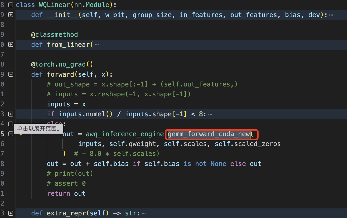
forward 函数部分用量化 kernel gemm_forward_cuda_new 替换原有的 pytorch 的 Linear 浮点线性层函数。主要代码如下所示:
4.2 packed_weight 函数分析
其中 pack_intweight 函数通过一系列的 reshape、transpose 等操作把量化后的权重(unpacked_qweight)重新排列和打包,以优化在 CUDA 内核中的高效计算。代码如下所示:
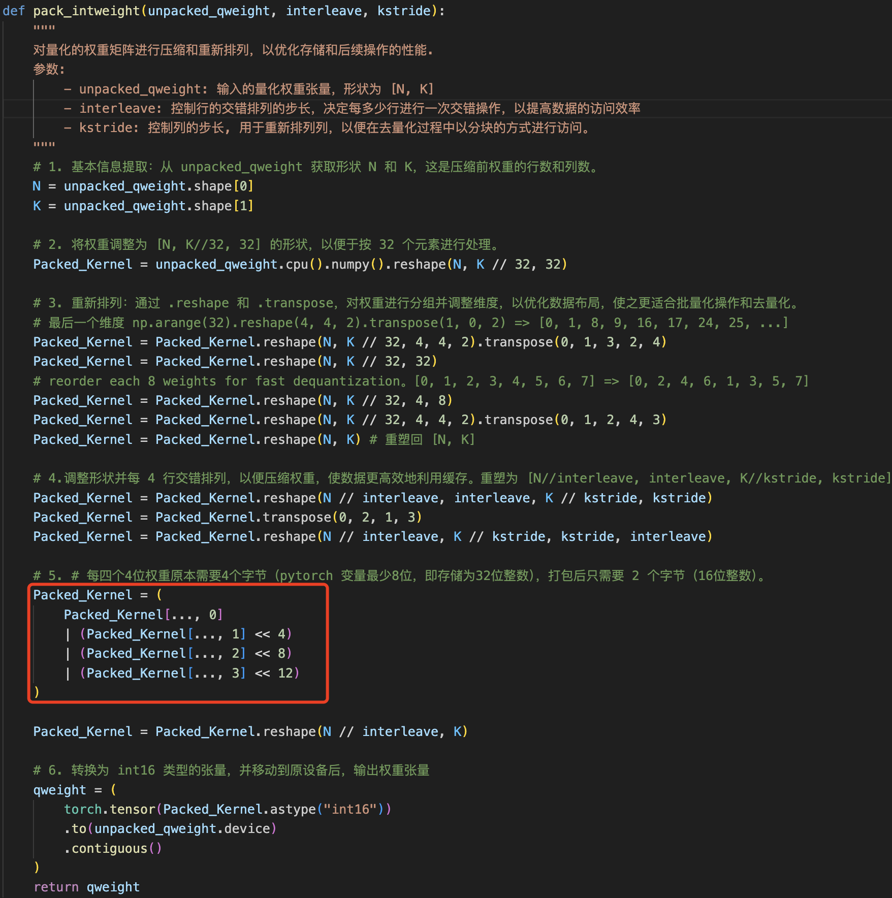
之所以需要这样做是因为原始的量化权重通常以较低位数(如 4 位)存储,但在 pytorch 标准张量中,每个元素通常占用至少 8 位或更多。通过将多个低位权重打包到一个较大的数据类型(如 int16)中,可以显著减少内存占用。虽然这个函数的目的大致是理解的,但是这么多过程的必要性操作是真不懂,pytorch 高手的操作张量是真的复杂。
先直接看下这个函数的效果吧,定义以下单元测试,并且测试代码运行成功。
def test_pack_intweight_edge_case(self):
    """
    测试特殊情况下的打包,如所有权重都是最大值15或最小值0。
    """
    N = 8
    K = 128
    interleave = 4
    kstride = 32

    # 测试所有权重为15的情况
    unpacked_qweight_max = torch.full((N, K), 15, dtype=torch.int64).to(self.device)
    packed_qweight_max = pack_intweight(unpacked_qweight_max, interleave, kstride)
    expected_packed_value_max = 15 | (15 << 4) | (15 << 8) | (15 << 12)
    self.assertTrue(torch.all(packed_qweight_max == expected_packed_value_max),
                    "Packed weight value mismatch when all weights are 15.")

    # 测试所有权重为0的情况
    unpacked_qweight_min = torch.zeros((N, K), dtype=torch.int64).to(self.device)
    packed_qweight_min = pack_intweight(unpacked_qweight_min, interleave, kstride)
    expected_packed_value_min = 0
    self.assertTrue(torch.all(packed_qweight_min == expected_packed_value_min),
                    "Packed weight value mismatch when all weights are 0.")
此外,我们的输入输出是这样的:
unpacked_qweight[0].shape
torch.Size([128])
unpacked_qweight_max[0]
tensor([15, 15, 15, 15, 15, 15, 15, 15, 15, 15, 15, 15, 15, 15, 15, 15, 15, 15,
        15, 15, 15, 15, 15, 15, 15, 15, 15, 15, 15, 15, 15, 15, 15, 15, 15, 15,
        15, 15, 15, 15, 15, 15, 15, 15, 15, 15, 15, 15, 15, 15, 15, 15, 15, 15,
        15, 15, 15, 15, 15, 15, 15, 15, 15, 15, 15, 15, 15, 15, 15, 15, 15, 15,
        15, 15, 15, 15, 15, 15, 15, 15, 15, 15, 15, 15, 15, 15, 15, 15, 15, 15,
        15, 15, 15, 15, 15, 15, 15, 15, 15, 15, 15, 15, 15, 15, 15, 15, 15, 15,
        15, 15, 15, 15, 15, 15, 15, 15, 15, 15, 15, 15, 15, 15, 15, 15, 15, 15,
        15, 15])

packed_qweight_max[0].shape
torch.Size([128])
packed_qweight_max[0]
array([65535, 65535, 65535, 65535, 65535, 65535, 65535, 65535, 65535,
       65535, 65535, 65535, 65535, 65535, 65535, 65535, 65535, 65535,
       65535, 65535, 65535, 65535, 65535, 65535, 65535, 65535, 65535,
       65535, 65535, 65535, 65535, 65535, 65535, 65535, 65535, 65535,
       65535, 65535, 65535, 65535, 65535, 65535, 65535, 65535, 65535,
       65535, 65535, 65535, 65535, 65535, 65535, 65535, 65535, 65535,
       65535, 65535, 65535, 65535, 65535, 65535, 65535, 65535, 65535,
       65535, 65535, 65535, 65535, 65535, 65535, 65535, 65535, 65535,
       65535, 65535, 65535, 65535, 65535, 65535, 65535, 65535, 65535,
       65535, 65535, 65535, 65535, 65535, 65535, 65535, 65535, 65535,
       65535, 65535, 65535, 65535, 65535, 65535, 65535, 65535, 65535,
       65535, 65535, 65535, 65535, 65535, 65535, 65535, 65535, 65535,
       65535, 65535, 65535, 65535, 65535, 65535, 65535, 65535, 65535,
       65535, 65535, 65535, 65535, 65535, 65535, 65535, 65535, 65535,
       65535, 65535])
很明显,在经过一系列权重打包处理后,4 个 INT4 大小的权重(实际存储为 8 位)的打包成 pytorch 的 INT16 类型,自然原来 INT4 权重的最大值由 15 变成 65535。权重
如果是 C++/CUDA 推理框架,是否也许要这步呢?
部分代码解释,如 << 左移位操作符。示例:value << num: value是运算对象,num 是要向左进行移位的位数,左移的时候在低位补0。其实左移n 位,就相当于乘以2 的 n 次方。比如 120 << 4 运算的结果是 1920 = 120 * 2^4。
4.3 vllm 的 量化 kernel
基础知识
1,uint4 数据类型
在 CUDA 编程中,uint4 是一种内置的向量类型,它由 4 个 32 位无符号整数(unsigned int)组成。其定义类似于下面的结构体:
typedef struct uint4 {
    // 每个元素 32 位:因此整个 uint4 类型占用 4×4 = 16 字节
    unsigned int x, y, z, w;
} uint4;
uint4 数据类型的特点:
- 向量化操作:uint4 常用于同时处理 4 个数据,便于进行并行计算或内存数据的打包和解包操作。
- 成员访问:可以通过
.x, .y, .z, .w分别访问每个分量。
2,S4 数据类型
S4 类型通常指的是用 4 位(bit)表示的有符号整数,也称为“4 位二补数”。 4 位能表示 2⁴ = 16 个不同的数值,但对于有符号数采用二补数表示,其取值范围是 –8 到 +7。一个 32 位整数中,可以存储 32/4 = 8 个 S4 数值,即将其“打包”成 8 个 S4 数据。
3,half 与 half2 数据类型
half: 16 位浮点数(也称为半精度浮点数),遵循 IEEE 754 binary16 格式。half2: CUDA 中的一种向量类型,它包含两个 half 数值。
kernel 代码解析
vllm 框架的 gemm 量化 kernel 实现代码是基于 llm_awq 仓库提供的量化 kernel 修改优化得到,代码地址在这里,kernel 推荐看 vllm 的实现,代码相对 awq 更为简洁和优雅易懂。值得注意的是,awq 量化 kernel 跟 smoothquant 有点不一样的是它没有量化激活,只量化了权重,因此量化 kernel 计算时得先对权重做反量化 dequantize 操作。
反量化操作的 kernel 函数是 dequantize_s4_to_fp16x2 (vllm/csrc/quantization/awq/dequantize.cuh),其作用是将一个存储为 32 位的 8 个 S4 格式量化数据转换为 4 个 half2(即 8 个 half 数值)的数据表示。转换过程中利用了内联 PTX 指令和特殊的立即数常量,以便高效地从 4 位整数编码转换到半精度浮点数。
带有注释(chatgpt o3 给出)的 dequantize_s4_to_fp16x2 代码如下所示。
#pragma once

#include <assert.h>
#include <cuda_fp16.h>
#include <stdint.h>

namespace vllm {
namespace awq {

/*
 * 该设备函数用于将一个 32 位整数(包含多个4位量化数据,S4 格式)转换为4个 half2 数据,
 * 最终以 uint4 类型返回(每个成员存放一个 half2,即2个 half,共4*2=8个 half 数值)。
 *
 * 注意:该实现仅在 CUDA 架构大于等于750时有效,否则会触发 assert(false)。
 */
__device__ uint4 dequantize_s4_to_fp16x2(uint32_t const& source) {
#if defined(__CUDA_ARCH__) && __CUDA_ARCH__ < 750
  // 若 CUDA 架构小于750,则不支持该转换
  assert(false);
#else
  // 定义返回结果变量 result,类型为 uint4,每个成员对应 half2 数据
  uint4 result;

  // 将 result 的内存视为一个 uint32_t 数组指针 h,共有4个 uint32_t 对应4个 half2 数据
  uint32_t* h = reinterpret_cast<uint32_t*>(&result);
  // 将输入 source 强制转换为 uint32_t,存入 i4s
  uint32_t const i4s = reinterpret_cast<uint32_t const&>(source);

  // 定义常量:
  // immLut:立即数查找表,具体位操作组合,用于后续 PTX 指令中的操作
  static constexpr uint32_t immLut = (0xf0 & 0xcc) | 0xaa;
  // BOTTOM_MASK:用于提取低位4位的掩码(每个32位整数中,低位部分)
  static constexpr uint32_t BOTTOM_MASK = 0x000f000f;
  // TOP_MASK:用于提取高位4位的掩码
  static constexpr uint32_t TOP_MASK = 0x00f000f0;
  // I4s_TO_F16s_MAGIC_NUM:转换时使用的魔数,通常用于将整数转换为浮点数格式的中间步骤
  static constexpr uint32_t I4s_TO_F16s_MAGIC_NUM = 0x64006400;

  // 注:整个转换过程仅需要1次移位指令,这是利用了寄存器打包格式,
  // 并且我们将整数视为无符号数,后续在 fp16 减法中进行了补偿处理。
  // 此外利用 sub 和 fma 指令具有相同吞吐量的特性,
  // 使得我们可以将 elt_23 和 elt_67 转换为 fp16 而无需提前移位到底部位。

  // 先将 i4s 右移 8 位,得到 top_i4s,用于后续提取 elt_45 和 elt_67,
  // 这样做有助于隐藏 RAW 依赖。
  const uint32_t top_i4s = i4s >> 8;

  // 使用 inline PTX 指令:使用 lop3.b32 指令提取 elt_01 部分
  // 计算:(i4s & BOTTOM_MASK) | I4s_TO_F16s_MAGIC_NUM,然后与 immLut 结合
  asm volatile("lop3.b32 %0, %1, %2, %3, %4;\n"
               : "=r"(h[0])
               : "r"(i4s), "n"(BOTTOM_MASK), "n"(I4s_TO_F16s_MAGIC_NUM),
                 "n"(immLut));

  // 提取 elt_23 部分:(i4s & TOP_MASK) | I4s_TO_F16s_MAGIC_NUM
  asm volatile("lop3.b32 %0, %1, %2, %3, %4;\n"
               : "=r"(h[1])
               : "r"(i4s), "n"(TOP_MASK), "n"(I4s_TO_F16s_MAGIC_NUM),
                 "n"(immLut));

  // 提取 elt_45 部分:(top_i4s & BOTTOM_MASK) | I4s_TO_F16s_MAGIC_NUM
  asm volatile("lop3.b32 %0, %1, %2, %3, %4;\n"
               : "=r"(h[2])
               : "r"(top_i4s), "n"(BOTTOM_MASK), "n"(I4s_TO_F16s_MAGIC_NUM),
                 "n"(immLut));

  // 提取 elt_67 部分:(top_i4s & TOP_MASK) | I4s_TO_F16s_MAGIC_NUM
  asm volatile("lop3.b32 %0, %1, %2, %3, %4;\n"
               : "=r"(h[3])
               : "r"(top_i4s), "n"(TOP_MASK), "n"(I4s_TO_F16s_MAGIC_NUM),
                 "n"(immLut));

  // 以下利用 inline PTX 进行后续转换,原因是不确定编译器是否会生成 float2half 指令,
  // 此处牺牲了一定可读性以确保性能和可靠性。

  // 定义常量:
  // FP16_TOP_MAGIC_NUM:代表 half2 {1024, 1024} 的魔数,用于后续转换(减去该值可使结果映射到正确范围)
  static constexpr uint32_t FP16_TOP_MAGIC_NUM = 0x64006400;
  // ONE_SIXTEENTH:代表 half2 {1/16, 1/16},用于缩放,即将整数转换为对应的半精度数
  static constexpr uint32_t ONE_SIXTEENTH = 0x2c002c00;
  // NEG_64:代表 half2 {-64, -64},用于补偿偏移,替代之前的 {-72, -72}
  static constexpr uint32_t NEG_64 = 0xd400d400;

  // 对每个提取出来的部分进行转换:
  // 对 elt_01:先用 sub.f16x2 指令将 h[0] 减去 FP16_TOP_MAGIC_NUM
  asm volatile("sub.f16x2 %0, %1, %2;\n"
               : "=r"(h[0])
               : "r"(h[0]), "r"(FP16_TOP_MAGIC_NUM));
  // 对 elt_23:使用 fma.rn.f16x2 指令,计算 h[1] * ONE_SIXTEENTH + NEG_64
  asm volatile("fma.rn.f16x2 %0, %1, %2, %3;\n"
               : "=r"(h[1])
               : "r"(h[1]), "r"(ONE_SIXTEENTH), "r"(NEG_64));
  // 对 elt_45:同样使用 sub.f16x2 指令
  asm volatile("sub.f16x2 %0, %1, %2;\n"
               : "=r"(h[2])
               : "r"(h[2]), "r"(FP16_TOP_MAGIC_NUM));
  // 对 elt_67:使用 fma.rn.f16x2 指令
  asm volatile("fma.rn.f16x2 %0, %1, %2, %3;\n"
               : "=r"(h[3])
               : "r"(h[3]), "r"(ONE_SIXTEENTH), "r"(NEG_64));

  // 返回转换结果,result 中包含了8个 half 数值(4个 half2)
  return result;
#endif
  // 如果编译器流到这里,说明缺少返回值,用 __builtin_unreachable() 消除警告
  __builtin_unreachable();
}

}  // namespace awq
}  // namespace vllm